PDF version (NAG web site
, 64-bit version, 64-bit version)
NAG Toolbox: nag_fit_1dspline_deriv (e02bc)
Purpose
nag_fit_1dspline_deriv (e02bc) evaluates a cubic spline and its first three derivatives from its B-spline representation.
Syntax
Description
nag_fit_1dspline_deriv (e02bc) evaluates the cubic spline
and its first three derivatives at a prescribed argument
. It is assumed that
is represented in terms of its B-spline coefficients
, for
and (augmented) ordered knot set
, for
,
(see
nag_fit_1dspline_knots (e02ba)),
i.e.,
Here
,
is the number of intervals of the spline and
denotes the normalized B-spline of degree
(order
) defined upon the knots
. The prescribed argument
must satisfy
At a simple knot (i.e., one satisfying ), the third derivative of the spline is in general discontinuous. At a multiple knot (i.e., two or more knots with the same value), lower derivatives, and even the spline itself, may be discontinuous. Specifically, at a point where (exactly) knots coincide (such a point is termed a knot of multiplicity ), the values of the derivatives of order , for , are in general discontinuous. (Here ; is not meaningful.) You must specify whether the value at such a point is required to be the left- or right-hand derivative.
The method employed is based upon:
| (i) |
carrying out a binary search for the knot interval containing the argument (see Cox (1978)), |
| (ii) |
evaluating the nonzero B-splines of orders , , and by recurrence (see Cox (1972) and Cox (1978)), |
| (iii) |
computing all derivatives of the B-splines of order by applying a second recurrence to these computed B-spline values (see de Boor (1972)), |
| (iv) |
multiplying the fourth-order B-spline values and their derivative by the appropriate B-spline coefficients, and summing, to yield the values of and its derivatives. |
nag_fit_1dspline_deriv (e02bc) can be used to compute the values and derivatives of cubic spline fits and interpolants produced by
nag_fit_1dspline_knots (e02ba).
If only values and not derivatives are required,
nag_fit_1dspline_eval (e02bb) may be used instead of
nag_fit_1dspline_deriv (e02bc), which takes about
longer than
nag_fit_1dspline_eval (e02bb).
References
Cox M G (1972) The numerical evaluation of B-splines J. Inst. Math. Appl. 10 134–149
Cox M G (1978) The numerical evaluation of a spline from its B-spline representation J. Inst. Math. Appl. 21 135–143
de Boor C (1972) On calculating with B-splines J. Approx. Theory 6 50–62
Parameters
Compulsory Input Parameters
- 1:
– double array
-
must be set to the value of the th member of the complete set of knots, , for .
Constraint:
the must be in nondecreasing order with
.
- 2:
– double array
-
The coefficient
of the B-spline , for . The remaining elements of the array are not referenced.
- 3:
– double scalar
-
The argument at which the cubic spline and its derivatives are to be evaluated.
Constraint:
.
- 4:
– int64int32nag_int scalar
-
Specifies whether left- or right-hand values of the spline and its derivatives are to be computed (see
Description). Left- or right-hand values are formed according to whether
left is equal or not equal to
.
If
does not coincide with a knot, the value of
left is immaterial.
If , right-hand values are computed.
If
, left-hand values are formed, regardless of the value of
left.
Optional Input Parameters
- 1:
– int64int32nag_int scalar
-
Default:
the dimension of the arrays
lamda,
c. (An error is raised if these dimensions are not equal.)
, where is the number of intervals of the spline (which is one greater than the number of interior knots, i.e., the knots strictly within the range to over which the spline is defined).
Constraint:
.
Output Parameters
- 1:
– double array
-
contains the value of the th derivative of the spline at the argument , for . Note that contains the value of the spline.
- 2:
– int64int32nag_int scalar
unless the function detects an error (see
Error Indicators and Warnings).
Error Indicators and Warnings
Errors or warnings detected by the function:
-
-
, i.e., the number of intervals is not positive.
-
-
Either
, i.e., the range over which
is defined is null or negative in length, or
x is an invalid argument, i.e.,
or
.
-
An unexpected error has been triggered by this routine. Please
contact
NAG.
-
Your licence key may have expired or may not have been installed correctly.
-
Dynamic memory allocation failed.
Accuracy
The computed value of
has negligible error in most practical situations. Specifically, this value has an
absolute error bounded in modulus by
, where
is the largest in modulus of
and
, and
is an integer such that
. If
and
are all of the same sign, then the computed value of
has
relative error bounded by
. For full details see
Cox (1978).
No complete error analysis is available for the computation of the derivatives of . However, for most practical purposes the absolute errors in the computed derivatives should be small.
Further Comments
The time taken is approximately linear in .
Note: the function does not test all the conditions on the knots given in the description of
lamda in
Arguments, since to do this would result in a computation time approximately linear in
instead of
. All the conditions are tested in
nag_fit_1dspline_knots (e02ba), however.
Example
Compute, at the arguments
,
,
,
,
,
,
,
the left- and right-hand values and first derivatives of the cubic spline defined over the interval having the interior knots
,
,
,
,
,
, the additional knots
,
,
,
,
,
,
,
, and the B-spline coefficients
,
,
,
,
,
,
,
,
,
.
The input data items (using the notation of
Arguments) comprise the following values in the order indicated:
|
|
| , |
for |
| , |
for |
| , |
for |
This example program is written in a general form that will enable the values and derivatives of a cubic spline having an arbitrary number of knots to be evaluated at a set of arbitrary points. Any number of datasets may be supplied.
The only changes required to the program relate to the dimensions of the arrays
lamda and
c.
Open in the MATLAB editor:
e02bc_example
function e02bc_example
fprintf('e02bc example results\n\n');
knots = [ 1 3 3 3 4 4];
ncap = size(knots,2) + 1;
ncap7 = ncap + 7;
lamda = zeros(ncap7,1);
lamda(5:ncap+3) = knots;
lamda(ncap+4:ncap7) = 6;
c = zeros(ncap7,1);
c(1:ncap+3) = [10 12 13 15 22 26 24 18 14 12];
left = int64(1);
right = int64(2);
k = 0;
for x = 0:0.2:6;
k = k+1;
[sl(:,k), ifail] = e02bc( ...
lamda, c, x, left);
[sr(:,k), ifail] = e02bc( ...
lamda, c, x, right);
end
x = 0:0.2:6;
fprintf('Left hand values and derivatives\n');
fprintf('%5s%12s%12s%11s%11s\n', 'x', 'spline', '1st deriv', ...
'2nd deriv', '3rd deriv');
sol = [ x; sl];
fprintf('%7.2f%11.4f%11.4f%11.4f%11.4f\n',sol(:,1:5:end));
fprintf('\nRight hand values and derivatives\n');
fprintf('%5s%12s%12s%11s%11s\n', 'x', 'spline', '1st deriv', ...
'2nd deriv', '3rd deriv');
sol = [ x; sr];
fprintf('%7.2f%11.4f%11.4f%11.4f%11.4f\n', sol(:,1:5:end));
fig1 = figure;
plot(x,sl(1,:),x,sl(2,:),x,sl(3,:),x,sl(4,:));
xlabel('x');
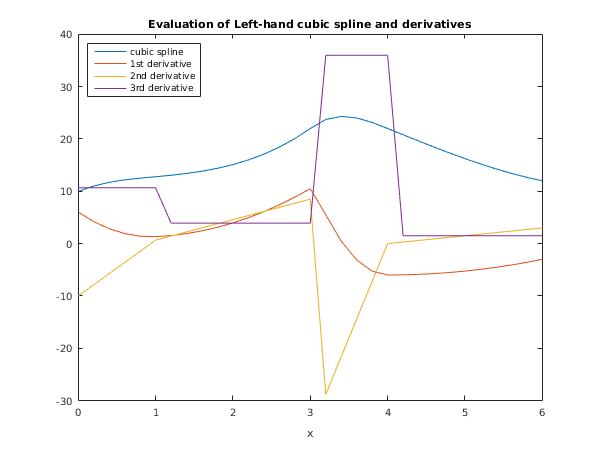
title('Evaluation of Left-hand cubic spline and derivatives');
legend('cubic spline', '1st derivative', '2nd derivative', ...
'3rd derivative', 'Location', 'NorthWest');
fig2 = figure;
plot(x,sr(1,:),x,sr(2,:),x,sr(3,:),x,sr(4,:));
xlabel('x');
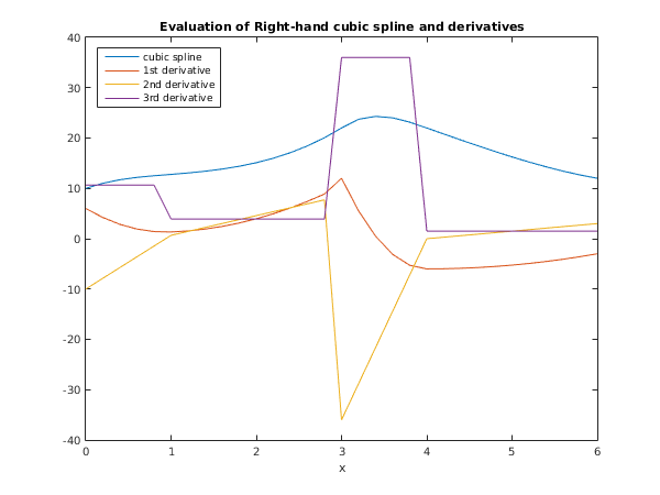
title('Evaluation of Right-hand cubic spline and derivatives');
legend('cubic spline', '1st derivative', '2nd derivative', ...
'3rd derivative', 'Location', 'NorthWest');
e02bc example results

Left hand values and derivatives
    x      spline   1st deriv  2nd deriv  3rd deriv
   0.00    10.0000     6.0000   -10.0000    10.6667
   1.00    12.7778     1.3333     0.6667    10.6667
   2.00    15.0972     3.9583     4.5833     3.9167
   3.00    22.0000    10.5000     8.5000     3.9167
   4.00    22.0000    -6.0000     0.0000    36.0000
   5.00    16.2500    -5.2500     1.5000     1.5000
   6.00    12.0000    -3.0000     3.0000     1.5000

Right hand values and derivatives
    x      spline   1st deriv  2nd deriv  3rd deriv
   0.00    10.0000     6.0000   -10.0000    10.6667
   1.00    12.7778     1.3333     0.6667     3.9167
   2.00    15.0972     3.9583     4.5833     3.9167
   3.00    22.0000    12.0000   -36.0000    36.0000
   4.00    22.0000    -6.0000     0.0000     1.5000
   5.00    16.2500    -5.2500     1.5000     1.5000
   6.00    12.0000    -3.0000     3.0000     1.5000
PDF version (NAG web site
, 64-bit version, 64-bit version)
© The Numerical Algorithms Group Ltd, Oxford, UK. 2009–2015