NAG Toolbox: nag_ode_ivp_stiff_imp_fulljac (d02ng)

Purpose

Syntax

Description

.
.
.
[...] = d02nv(...);
[...] = d02ns(...);
[..., ifail] = d02ng(...);
if (ifail ~= 1 and ifail < 14) 
  [...] = d02ny(...);
end
.
.
.

References

Parameters

Compulsory Input Parameters

1:     $\mathrm{t}$ – double scalar

$t$, the value of the independent variable. The input value of t is used only on the first call as the initial point of the integration.

2:     $\mathrm{tout}$ – double scalar

The next value of $t$ at which a computed solution is desired. For the initial $t$, the input value of tout is used to determine the direction of integration. Integration is permitted in either direction (see also itask).

Constraint: $\mathbf{tout}\ne \mathbf{t}$.

3:     $\mathrm{y}\left(\mathbf{neq}\right)$ – double array

The values of the dependent variables (solution). On the first call the first neq elements of y must contain the vector of initial values.

4:     $\mathrm{ydot}\left(\mathbf{neq}\right)$ – double array

If $\mathbf{lderiv}\left(1\right)=\mathit{true}$, ydot must contain approximations to the time derivatives $y^{\prime }$ of the vector $y$.

If $\mathbf{lderiv}\left(1\right)=\mathit{false}$, ydot need not be set on entry.

5:     $\mathrm{rwork}\left(50+4\times \mathbf{neq}\right)$ – double array

6:     $\mathrm{rtol}\left(:\right)$ – double array

The dimension of the array rtol must be at least $1$ if $\mathbf{itol}=1$ or $2$, and at least $\mathbf{neq}$ otherwise

The relative local error tolerance.

Constraint: $\mathbf{rtol}\left(i\right)\ge 0.0$ for all relevant $i$ (see itol).

7:     $\mathrm{atol}\left(:\right)$ – double array

The dimension of the array atol must be at least $1$ if $\mathbf{itol}=1$ or $3$, and at least $\mathbf{neq}$ otherwise

The absolute local error tolerance.

Constraint: $\mathbf{atol}\left(i\right)\ge 0.0$ for all relevant $i$ (see itol).

8:     $\mathrm{itol}$ – int64int32nag_int scalar

A value to indicate the form of the local error test. itol indicates to nag_ode_ivp_stiff_imp_fulljac (d02ng) whether to interpret either or both of rtol or atol as a vector or a scalar. The error test to be satisfied is $‖e_i/w_i‖<1.0$, where $w_i$ is defined as follows:

itol	rtol	atol	$w_i$
1	scalar	scalar	$\mathbf{rtol}\left(1\right)\times \left|y_i\right|+\mathbf{atol}\left(1\right)$
2	scalar	vector	$\mathbf{rtol}\left(1\right)\times \left|y_i\right|+\mathbf{atol}\left(i\right)$
3	vector	scalar	$\mathbf{rtol}\left(i\right)\times \left|y_i\right|+\mathbf{atol}\left(1\right)$
4	vector	vector	$\mathbf{rtol}\left(i\right)\times \left|y_i\right|+\mathbf{atol}\left(i\right)$

$e_i$ is an estimate of the local error in $y_i$, computed internally, and the choice of norm to be used is defined by a previous call to an integrator setup function.

Constraint: $\mathbf{itol}=1$, $2$, $3$ or $4$.

9:     $\mathrm{inform}\left(23\right)$ – int64int32nag_int array

10:   $\mathrm{resid}$ – function handle or string containing name of m-file

resid must evaluate the residual

$$r=g\left(t,y\right)-A\left(t,y\right)y^{\prime }$$

in one case and

$$r=-A\left(t,y\right)y^{\prime }$$

in another.

[r, ires] = resid(neq, t, y, ydot, ires)

Input Parameters

1:     $\mathrm{neq}$ – int64int32nag_int scalar

The number of equations being solved.

2:     $\mathrm{t}$ – double scalar

$t$, the current value of the independent variable.

3:     $\mathrm{y}\left(\mathbf{neq}\right)$ – double array

The value of $y_{\mathit{i}}$, for $\mathit{i}=1,2,\dots ,\mathbf{neq}$.

4:     $\mathrm{ydot}\left(\mathbf{neq}\right)$ – double array

The value of $y_{\mathit{i}}^{\prime }$, for $\mathit{i}=1,2,\dots ,\mathbf{neq}$, at $t$.

5:     $\mathrm{ires}$ – int64int32nag_int scalar

The form of the residual that must be returned in array r.

$\mathbf{ires}=-1$

The residual defined in equation (2) must be returned.

$\mathbf{ires}=1$

The residual defined in equation (1) must be returned.

Output Parameters

1:     $\mathrm{r}\left(\mathbf{neq}\right)$ – double array

$\mathbf{r}\left(\mathit{i}\right)$ must contain the $\mathit{i}$th component of $r$, for $\mathit{i}=1,2,\dots ,\mathbf{neq}$, where

$$r=g\left(t,y\right)-A\left(t,y\right)y^{\prime }$$

(1)

or

$$r=-A\left(t,y\right)y^{\prime }$$

(2)

and where the definition of $r$ is determined by the input value of ires.

2:     $\mathrm{ires}$ – int64int32nag_int scalar

Should be unchanged unless one of the following actions is required of the integrator, in which case ires should be set accordingly.

$\mathbf{ires}=2$

Indicates to the integrator that control should be passed back immediately to the calling (sub)program with the error indicator set to $\mathbf{ifail}=\mathbf{11}$.

$\mathbf{ires}=3$

Indicates to the integrator that an error condition has occurred in the solution vector, its time derivative or in the value of $t$. The integrator will use a smaller time step to try to avoid this condition. If this is not possible, the integrator returns to the calling (sub)program with the error indicator set to $\mathbf{ifail}=\mathbf{7}$.

$\mathbf{ires}=4$

Indicates to the integrator to stop its current operation and to enter monitr immediately with argument $\mathbf{imon}=-2$.

11:   $\mathrm{ysav}\left(\mathit{ldysav},\mathbf{sdysav}\right)$ – double array

ldysav, the first dimension of the array, must satisfy the constraint $\mathit{ldysav}\ge \mathbf{neq}$.

An appropriate value for sdysav is described in the specifications of the integrator setup functions nag_ode_ivp_stiff_dassl (d02mv), nag_ode_ivp_stiff_bdf (d02nv) and nag_ode_ivp_stiff_blend (d02nw). This value must be the same as that supplied to the integrator setup function.

12:   $\mathrm{jac}$ – function handle or string containing name of m-file

jac must evaluate the Jacobian of the system. If this option is not required, the actual argument for jac must be the string nag_ode_ivp_stiff_imp_fulljac_dummy_jac (d02ngz). (nag_ode_ivp_stiff_imp_fulljac_dummy_jac (d02ngz) is included in the NAG Toolbox.) You must indicate to the integrator whether this option is to be used by setting the argument jceval appropriately in a call to the full linear algebra setup function nag_ode_ivp_stiff_fulljac_setup (d02ns).

First we must define the system of nonlinear equations which is solved internally by the integrator. The time derivative, $y^{\prime }$, generated internally, has the form

$$y^{\prime }=\left(y-z\right)/\left(hd\right)\text{,}$$

where $h$ is the current step size and $d$ is a argument that depends on the integration method in use. The vector $y$ is the current solution and the vector $z$ depends on information from previous time steps. This means that $\frac{d}{d{y}^{\prime }}\left(\text{ }\right)=\left(hd\right)\frac{d}{dy}\left(\text{ }\right)$. The system of nonlinear equations that is solved has the form

$$A\left(t,y\right)y^{\prime }-g\left(t,y\right)=0$$

but it is solved in the form

$$r\left(t,y\right)=0\text{,}$$

where $r$ is the function defined by

$$r\left(t,y\right)=\left(hd\right)\left(A\left(t,y\right)\left(y-z\right)/\left(hd\right)-g\left(t,y\right)\right)\text{.}$$

It is the Jacobian matrix $\frac{\partial r}{\partial y}$ that you must supply in jac as follows:

$$\frac{\partial r_i}{\partial y_j}=a_{ij}\left(t,y\right)+\left(hd\right)\frac{\partial }{\partial y_j}\left(\sum _{k=1}^{\mathbf{neq}}{a}_{ik}\left(t,y\right)y_k^{\prime }-g_i\left(t,y\right)\right)\text{.}$$

[p] = jac(neq, t, y, ydot, h, d, p)

Input Parameters

1:     $\mathrm{neq}$ – int64int32nag_int scalar

The number of equations being solved.

2:     $\mathrm{t}$ – double scalar

$t$, the current value of the independent variable.

3:     $\mathrm{y}\left(\mathbf{neq}\right)$ – double array

$y_{\mathit{i}}$, for $\mathit{i}=1,2,\dots ,\mathbf{neq}$, the current solution component.

4:     $\mathrm{ydot}\left(\mathbf{neq}\right)$ – double array

The derivative of the solution at the current point $t$.

5:     $\mathrm{h}$ – double scalar

The current step size.

6:     $\mathrm{d}$ – double scalar

The argument $d$ which depends on the integration method.

7:     $\mathrm{p}\left(\mathbf{neq},\mathbf{neq}\right)$ – double array

Is set to zero.

Output Parameters

1:     $\mathrm{p}\left(\mathbf{neq},\mathbf{neq}\right)$ – double array

$\mathbf{p}\left(\mathit{i},\mathit{j}\right)$ must contain $\frac{\partial r_{\mathit{i}}}{\partial y_{\mathit{j}}}$, for $\mathit{i}=1,2,\dots ,\mathbf{neq}$ and $\mathit{j}=1,2,\dots ,\mathbf{neq}$.

Only the nonzero elements of this array need be set, since it is preset to zero before the call to jac.

13:   $\mathrm{wkjac}\left(\mathit{nwkjac}\right)$ – double array

nwkjac, the dimension of the array, must satisfy the constraint $\mathit{nwkjac}\ge \mathit{ldysav}\times \left(\mathit{ldysav}+1\right)$.

This value must be the same as that supplied to the linear algebra setup function nag_ode_ivp_stiff_fulljac_setup (d02ns).

Constraint: $\mathit{nwkjac}\ge \mathit{ldysav}\times \left(\mathit{ldysav}+1\right)$.

14:   $\mathrm{monitr}$ – function handle or string containing name of m-file

monitr performs tasks requested by you. If this option is not required, then the actual argument for monitr must be the string nag_ode_ivp_stiff_exp_fulljac_dummy_monit (d02nby). (nag_ode_ivp_stiff_exp_fulljac_dummy_monit (d02nby) is included in the NAG Toolbox.)

[hnext, y, imon, inln, hmin, hmax] = monitr(neq, ldysav, t, hlast, hnext, y, ydot, ysav, r, acor, imon, hmin, hmax, nqu)

Input Parameters

1:     $\mathrm{neq}$ – int64int32nag_int scalar

The number of equations being solved.

2:     $\mathrm{ldysav}$ – int64int32nag_int scalar

An upper bound on the number of equations to be solved.

3:     $\mathrm{t}$ – double scalar

The current value of the independent variable.

4:     $\mathrm{hlast}$ – double scalar

The last step size successfully used by the integrator.

5:     $\mathrm{hnext}$ – double scalar

The step size that the integrator proposes to take on the next step.

6:     $\mathrm{y}\left(\mathbf{neq}\right)$ – double array

$y$, the values of the dependent variables evaluated at $t$.

7:     $\mathrm{ydot}\left(\mathbf{neq}\right)$ – double array

The time derivatives $y^{\prime }$ of the vector $y$.

8:     $\mathrm{ysav}\left(\mathit{ldysav},\mathit{sdysav}\right)$ – double array

Workspace to enable you to carry out interpolation using either of the functions nag_ode_ivp_stiff_nat_interp (d02xj) or nag_ode_ivp_stiff_c1_interp (d02xk).

9:     $\mathrm{r}\left(\mathbf{neq}\right)$ – double array

If $\mathbf{imon}=0$ and $\mathbf{inln}=3$, then the first neq elements contain the residual vector $A\left(t,y\right)y^{\prime }-g\left(t,y\right)$.

10:   $\mathrm{acor}\left(\mathbf{neq},2\right)$ – double array

With $\mathbf{imon}=1$, $\mathbf{acor}\left(i,1\right)$ contains the weight used for the $i$th equation when the norm is evaluated, and $\mathbf{acor}\left(i,2\right)$ contains the estimated local error for the $i$th equation. The scaled local error at the end of a timestep may be obtained by calling the double function nag_ode_ivp_stiff_errest (d02za) as follows:

 [errloc, ifail] = d02za(acor(1:neq,2), acor(1:neq,1));
 % Check ifail before proceeding 

11:   $\mathrm{imon}$ – int64int32nag_int scalar

A flag indicating under what circumstances monitr was called:

$\mathbf{imon}=-2$

Entry from the integrator after $\mathbf{ires}=4$ (set in resid) caused an early termination (this facility could be used to locate discontinuities).

$\mathbf{imon}=-1$

The current step failed repeatedly.

$\mathbf{imon}=0$

Entry after a call to the internal nonlinear equation solver (see inln).

$\mathbf{imon}=1$

The current step was successful.

12:   $\mathrm{hmin}$ – double scalar

The minimum step size to be taken on the next step.

13:   $\mathrm{hmax}$ – double scalar

The maximum step size to be taken on the next step.

14:   $\mathrm{nqu}$ – int64int32nag_int scalar

The order of the integrator used on the last step. This is supplied to enable you to carry out interpolation using either of the functions nag_ode_ivp_stiff_nat_interp (d02xj) or nag_ode_ivp_stiff_c1_interp (d02xk).

Output Parameters

1:     $\mathrm{hnext}$ – double scalar

The next step size to be used. If this is different from the input value, then imon must be set to $4$.

2:     $\mathrm{y}\left(\mathbf{neq}\right)$ – double array

These values must not be changed unless imon is set to $2$.

3:     $\mathrm{imon}$ – int64int32nag_int scalar

May be reset to determine subsequent action in nag_ode_ivp_stiff_imp_fulljac (d02ng).

$\mathbf{imon}=-2$

Integration is to be halted. A return will be made from the integrator to the calling (sub)program with $\mathbf{ifail}=\mathbf{12}$.

$\mathbf{imon}=-1$

Allow the integrator to continue with its own internal strategy. The integrator will try up to three restarts unless $\mathbf{imon}\ne -1$ on exit.

$\mathbf{imon}=0$

Return to the internal nonlinear equation solver, where the action taken is determined by the value of inln (see inln).

$\mathbf{imon}=1$

Normal exit to the integrator to continue integration.

$\mathbf{imon}=2$

Restart the integration at the current time point. The integrator will restart from order $1$ when this option is used. The solution y, provided by monitr, will be used for the initial conditions.

$\mathbf{imon}=3$

Try to continue with the same step size and order as was to be used before the call to monitr. hmin and hmax may be altered if desired.

$\mathbf{imon}=4$

Continue the integration but using a new value of hnext and possibly new values of hmin and hmax.

4:     $\mathrm{inln}$ – int64int32nag_int scalar

The action to be taken by the internal nonlinear equation solver when monitr is exited with $\mathbf{imon}=0$. By setting $\mathbf{inln}=3$ and returning to the integrator, the residual vector is evaluated and placed in the array r, and then monitr is called again. At present this is the only option available: inln must not be set to any other value.

5:     $\mathrm{hmin}$ – double scalar

The minimum step size to be used. If this is different from the input value, then imon must be set to $3$ or $4$.

6:     $\mathrm{hmax}$ – double scalar

The maximum step size to be used. If this is different from the input value, then imon must be set to $3$ or $4$. If hmax is set to zero, no limit is assumed.

15:   $\mathrm{lderiv}\left(2\right)$ – logical array

$\mathbf{lderiv}\left(1\right)$ must be set to true if you have supplied both an initial $y$ and an initial $y^{\prime }$. $\mathbf{lderiv}\left(1\right)$ must be set to false if only the initial $y$ has been supplied.

$\mathbf{lderiv}\left(2\right)$ must be set to true if the integrator is to use a modified Newton method to evaluate the initial $y$ and $y^{\prime }$. Note that $y$ and $y^{\prime }$, if supplied, are used as initial estimates. This method involves taking a small step at the start of the integration, and if $\mathbf{itask}=6$ on entry, t and tout will be set to the result of taking this small step. $\mathbf{lderiv}\left(2\right)$ must be set to false if the integrator is to use functional iteration to evaluate the initial $y$ and $y^{\prime }$, and if this fails a modified Newton method will then be attempted. $\mathbf{lderiv}\left(2\right)=\mathit{true}$ is recommended if there are implicit equations or the initial $y$ and $y^{\prime }$ are zero.

16:   $\mathrm{itask}$ – int64int32nag_int scalar

The task to be performed by the integrator.

$\mathbf{itask}=1$

Normal computation of output values of $y\left(t\right)$ at $t=\mathbf{tout}$ (by overshooting and interpolating).

$\mathbf{itask}=2$

Take one step only and return.

$\mathbf{itask}=3$

Stop at the first internal integration point at or beyond $t=\mathbf{tout}$ and return.

$\mathbf{itask}=4$

Normal computation of output values of $y\left(t\right)$ at $t=\mathbf{tout}$ but without overshooting $t=\mathbf{tcrit}$. tcrit must be specified as an option in one of the integrator setup functions before the first call to the integrator, or specified in the optional input function before a continuation call. tcrit may be equal to or beyond tout, but not before it, in the direction of integration.

$\mathbf{itask}=5$

Take one step only and return, without passing tcrit. tcrit must be specified as under $\mathbf{itask}=4$.

$\mathbf{itask}=6$

The integrator will solve for the initial values of $y$ and $y^{\prime }$ only and then return to the calling (sub)program without doing the integration. This option can be used to check the initial values of $y$ and $y^{\prime }$. Functional iteration or a ‘small’ backward Euler method used in conjunction with a damped Newton iteration is used to calculate these values (see lderiv). Note that if a backward Euler step is used then the value of $t$ will have been advanced a short distance from the initial point.

Note:  if nag_ode_ivp_stiff_imp_fulljac (d02ng) is recalled with a different value of itask (and tout altered), then the initialization procedure is repeated, possibly leading to different initial conditions.

Constraint: $1\le \mathbf{itask}\le 6$.

17:   $\mathrm{itrace}$ – int64int32nag_int scalar

The level of output that is printed by the integrator. itrace may take the value $-1$, $0$, $1$, $2$ or $3$.

$\mathbf{itrace}<-1$

$-1$ is assumed and similarly if $\mathbf{itrace}>3$, then $3$ is assumed.

$\mathbf{itrace}=-1$

No output is generated.

$\mathbf{itrace}=0$

Only warning messages are printed on the current error message unit (see nag_file_set_unit_error (x04aa)).

$\mathbf{itrace}>0$

Warning messages are printed as above, and on the current advisory message unit (see nag_file_set_unit_advisory (x04ab)) output is generated which details Jacobian entries, the nonlinear iteration and the time integration. The advisory messages are given in greater detail the larger the value of itrace.

Optional Input Parameters

1:     $\mathrm{neq}$ – int64int32nag_int scalar

Default: the dimension of the arrays y, ydot and the first dimension of the array ysav. (An error is raised if these dimensions are not equal.)

The number of differential equations to be solved.

Constraint: $\mathbf{neq}\ge 1$.

2:     $\mathrm{sdysav}$ – int64int32nag_int scalar

Default: the second dimension of the array ysav.

An appropriate value for sdysav is described in the specifications of the integrator setup functions nag_ode_ivp_stiff_dassl (d02mv), nag_ode_ivp_stiff_bdf (d02nv) and nag_ode_ivp_stiff_blend (d02nw). This value must be the same as that supplied to the integrator setup function.

Output Parameters

1:     $\mathrm{t}$ – double scalar

The value at which the computed solution $y$ is returned (usually at tout).

2:     $\mathrm{tout}$ – double scalar

Normally unchanged. However, when $\mathbf{itask}=6$, then tout contains the value of t at which initial values have been computed without performing any integration. See descriptions of itask and lderiv.

3:     $\mathrm{y}\left(\mathbf{neq}\right)$ – double array

The computed solution vector, evaluated at t (usually $\mathbf{t}=\mathbf{tout}$).

4:     $\mathrm{ydot}\left(\mathbf{neq}\right)$ – double array

The time derivatives $y^{\prime }$ of the vector $y$ at the last integration point.

5:     $\mathrm{rwork}\left(50+4\times \mathbf{neq}\right)$ – double array

6:     $\mathrm{inform}\left(23\right)$ – int64int32nag_int array

7:     $\mathrm{ysav}\left(\mathit{ldysav},\mathbf{sdysav}\right)$ – double array

Communication array, used to store information between calls to nag_ode_ivp_stiff_imp_fulljac (d02ng).

8:     $\mathrm{wkjac}\left(\mathit{nwkjac}\right)$ – double array

$\mathit{nwkjac}=\mathit{ldysav}\times \left(\mathit{ldysav}+1\right)$.

Communication array, used to store information between calls to nag_ode_ivp_stiff_imp_fulljac (d02ng).

9:     $\mathrm{lderiv}\left(2\right)$ – logical array

$\mathbf{lderiv}\left(1\right)$ is normally unchanged. However if $\mathbf{itask}=6$ and internal initialization was successful then $\mathbf{lderiv}\left(1\right)=\mathit{true}$.

$\mathbf{lderiv}\left(2\right)=\mathit{true}$, if implicit equations were detected. Otherwise $\mathbf{lderiv}\left(2\right)=\mathit{false}$.

10:   $\mathrm{ifail}$ – int64int32nag_int scalar

$\mathbf{ifail}=\mathbf{0}$ unless the function detects an error (see Error Indicators and Warnings).

Error Indicators and Warnings

Cases prefixed with W are classified as warnings and do not generate an error of type NAG:error_n. See nag_issue_warnings.

   $\mathbf{ifail}=1$

An illegal input was detected on entry, or after an internal call to monitr. If $\mathbf{itrace}>-1$, then the form of the error will be detailed on the current error message unit (see nag_file_set_unit_error (x04aa)).

   $\mathbf{ifail}=2$

The maximum number of steps specified has been taken (see the description of optional inputs in the integrator setup functions and the optional input continuation function, nag_ode_ivp_stiff_contin (d02nz)).

   $\mathbf{ifail}=3$

With the given values of rtol and atol no further progress can be made across the integration range from the current point t. The components $\mathbf{y}\left(1\right),\mathbf{y}\left(2\right),\dots ,\mathbf{y}\left(\mathbf{neq}\right)$ contain the computed values of the solution at the current point t.

   $\mathbf{ifail}=4$

There were repeated error test failures on an attempted step, before completing the requested task, but the integration was successful as far as t. The problem may have a singularity, or the local error requirements may be inappropriate.

   $\mathbf{ifail}=5$

There were repeated convergence test failures on an attempted step, before completing the requested task, but the integration was successful as far as t. This may be caused by an inaccurate Jacobian matrix or one which is incorrectly computed.

   $\mathbf{ifail}=6$

Some error weight $w_i$ became zero during the integration (see the description of itol). Pure relative error control ($\mathbf{atol}\left(i\right)=0.0$) was requested on a variable (the $i$th) which has now vanished. The integration was successful as far as t.

   $\mathbf{ifail}=7$

resid set its error flag ($\mathbf{ires}=3$) continually despite repeated attempts by the integrator to avoid this.

   $\mathbf{ifail}=8$

$\mathbf{lderiv}\left(1\right)=\mathit{false}$ on entry but the internal initialization function was unable to initialize $y^{\prime }$ (more detailed information may be directed to the current error message unit, see nag_file_set_unit_error (x04aa)).

   $\mathbf{ifail}=9$

A singular Jacobian $\frac{\partial r}{\partial y}$ has been encountered. You should check the problem formulation and Jacobian calculation.

   $\mathbf{ifail}=10$

An error occurred during Jacobian formulation or back-substitution (a more detailed error description may be directed to the current error message unit, see nag_file_set_unit_error (x04aa)).

W  $\mathbf{ifail}=11$

resid signalled the integrator to halt the integration and return ($\mathbf{ires}=2$). Integration was successful as far as t.

W  $\mathbf{ifail}=12$

monitr set $\mathbf{imon}=-2$ and so forced a return but the integration was successful as far as t.

W  $\mathbf{ifail}=13$

The requested task has been completed, but it is estimated that a small change in rtol and atol is unlikely to produce any change in the computed solution. (Only applies when you are not operating in one step mode, that is when $\mathbf{itask}\ne 2$ or $5$.)

   $\mathbf{ifail}=14$

The values of rtol and atol are so small that nag_ode_ivp_stiff_imp_fulljac (d02ng) is unable to start the integration.

   $\mathbf{ifail}=15$

The linear algebra setup function nag_ode_ivp_stiff_fulljac_setup (d02ns) was not called before the call to nag_ode_ivp_stiff_imp_fulljac (d02ng).

   $\mathbf{ifail}=-99$

An unexpected error has been triggered by this routine. Please contact NAG.

   $\mathbf{ifail}=-399$

Your licence key may have expired or may not have been installed correctly.

   $\mathbf{ifail}=-999$

Dynamic memory allocation failed.

Accuracy

Further Comments

Example

Open in the MATLAB editor: d02ng_example

function d02ng_example


fprintf('d02ng example results\n\n');

% switch for diagnostics output
istat  = 1;

% Initialize setup variables and arrays.
neq    = int64(3);
neqmax = neq;
maxord = int64(5);
sdysav = maxord+1;
petzld = false;
tcrit  = 0;
hmin   = 1.0e-10;
hmax   = 10;
h0     = 0;
maxstp = int64(200);
mxhnil = int64(5);

const = zeros(6, 1);
rwork = zeros(50+4*neq, 1);

% d02nv is a setup routine to be called prior to d02ng.
[const, rwork, ifail] = ...
d02nv( ...
       neqmax, sdysav, maxord, 'Functional', petzld, ...
       const, tcrit, hmin, hmax, h0, maxstp, mxhnil, 'Average-L2', rwork);

nwkjac = int64(neq*(neq+1));
% Numerical Jacobian.
[rwork, ifail] = d02ns( ...
                        neq, neqmax, 'Numerical', nwkjac, rwork);

% Initialize integration variables and arrays

sol   = zeros(neq, 1);
wkjac = zeros(nwkjac, 1);
ysave = zeros(neq, sdysav);
ydot  = zeros(neq, 1);
inform(1:23) = int64(0);
algequ = false(neq, 1);

% Integrate to tout by overshooting tout in one step mode (itask=2);
% use BDF with functional iteration; use vector tolerances (itol=4);
% dummy d02nbz and d02nby are used for Jacobian and monitor functions.
t    = 0;
tout = 0.1;
itask  = int64(2);
itrace = int64(0);
y      = [1; 0; 0];
lderiv = [false; false];
itol = int64(4);
rtol = [0.0001; 0.001; 0.0001];
atol = [1e-07; 1e-08; 1e-07];

% Output header and initial results.
fprintf('    x             y_1            y_2            y_3\n');
fprintf('%8.3f       %8.4f       %8.6f       %8.4f\n',t,y);

% Prepare to store results for plotting.
ncall = 1;
tkeep = t;
ykeep = y;
tstep = 0.02;

% xout is intermediate output points for printing solution.
iout = 1;
xout = iout*tstep;

while t < tout
  % Calculate solution at this point.
  [t, tout, y, ydot, rwork, inform, ysave, wkjac, lderiv, ifail] = ...
  d02ng( ...
         t, tout, y, ydot, rwork, rtol, atol, itol, inform, @resid, ...
         ysave, 'd02ngz', wkjac, 'd02nby', lderiv, itask, itrace);
  if (t<tstep)
    ncall = ncall+1;
    ykeep(:,ncall) = y;
    tkeep(ncall) = t;
  elseif (xout <= t)
    % Passed over intermediate output point (xout)
    % Interpolate the solution to get its value at xout.
    [hu, h, tcur, tolsf, nst, nre, nje, nqu, nq, niter, imxer, algequ, ...
     ifail] = d02ny( ...
                     neq, neqmax, rwork, inform);
    [sol, ifail] = d02xj( ...
                          xout, neq, ysave, neq, tcur, ...
                          nqu, hu, h, 'sdysav', sdysav);

    % Accumulate results for plotting.
    ncall = ncall + 1;
    ykeep(:,ncall) = sol;
    tkeep(ncall) = xout;
    % output intermediate results
    fprintf('%8.3f       %8.4f       %8.6f       %8.4f\n',xout,sol);

    % Bump the counter for the next output point.
    iout = iout + 1;
    xout = iout*tstep;
  end
end

% Output some statistics, if required.
if istat == 1
  [hu, h, tcur, tolsf, nst, nre, nje, nqu, nq, niter, imxer, algequ, ifail] ...
  = d02ny( ...
           neq, neqmax, rwork, inform);
  fprintf('\nDiagnostic information\n integration status:\n');
  fprintf('   last and next step sizes = %8.5f, %8.5f\n',hu, h);
  fprintf('   integration stopped at x = %8.5f\n',tcur);
  fprintf(' algorithm statistics:\n');
  fprintf('   number of time-steps and Newton iterations  = %5d %5d\n', ...
          nst,niter);
  fprintf('   number of residual and jacobian evaluations = %5d %5d\n', ...
          nre,nje);
  fprintf('   order of method last used and next to use   = %5d %5d\n', ...
          nqu,nq);
  fprintf('   component with largest error                = %5d\n',imxer);
end
% Plot results.
fig1 = figure;
display_plot(tkeep, ykeep)


function [r, ires] = resid(neq, t, y, ydot, ires)
  % Evaluate the residual.
  r(1:3) = -ydot(1:3);
  if ires == 1
    r(1) = -0.04*y(1) + 1.0e4*y(2)*y(3) + r(1);
    r(2) =  0.04*y(1) - 1.0e4*y(2)*y(3) - 3.0e7*y(2)*y(2) + r(2);
    r(3) =  3.0e7*y(2)*y(2) + r(3);
  end

function display_plot(x,y)
  % Formatting for title and axis labels.
  % Plot one of the curves and then add the other two.
  hline3 = plot(x, y(3,:));
  hold on;
  [haxes, hline1, hline2] = plotyy(x, 100*y(2,:), x, y(1,:));
  % Set the axis limits and the tick specifications to beautify the plot.
  set(haxes(1), 'YLim', [0.0 0.0045]);
  set(haxes(1), 'XMinorTick', 'on', 'YMinorTick', 'on');
  set(haxes(1), 'YTick', [0:0.001:0.004]);
  set(haxes(2), 'YLim', [0.995 1.006]);
  set(haxes(2), 'YMinorTick', 'on');
  set(haxes(2), 'YTick', [0.995:0.002:1.005]);
  set(haxes(1), 'XLim', [-0.005 0.1]);
  set(haxes(2), 'XLim', [-0.005 0.1]);
  set(gca, 'box', 'off'); % no ticks on opposite axes.
  % Add title.
  ht = title({'Stiff Robertson Problem:','BDF and Functional Iteration'});
  set(ht,'Position',[0.05,0.004,0.0]);
  % Label the x axis, and both y axes.
  xlabel('x');
  ylabel(haxes(1), 'Solution (100*b,c)');
  ylabel(haxes(2), 'Solution (a)');
  % Add a legend.
  legend('c', '100*b', 'a', 'Location', 'Best');
  % Set some features of the three lines
  set(hline1,'Linewidth',0.5,'Marker','+','LineStyle','-','Color','red');
  set(hline2,'Linewidth',0.5,'Marker','*','LineStyle',':','Color','blue');
  set(hline3,'Linewidth',0.5,'Marker','x','LineStyle','--','Color','green');
  hold off;

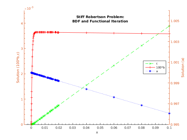
d02ng example results

    x             y_1            y_2            y_3
   0.000         1.0000       0.000000         0.0000
   0.020         0.9992       0.000036         0.0008
   0.040         0.9984       0.000036         0.0016
   0.060         0.9976       0.000036         0.0023
   0.080         0.9969       0.000036         0.0031
   0.100         0.9961       0.000036         0.0039

Diagnostic information
 integration status:
   last and next step sizes =  0.00027,  0.00053
   integration stopped at x =  0.10016
 algorithm statistics:
   number of time-steps and Newton iterations  =   244     0
   number of residual and jacobian evaluations =   809     0
   order of method last used and next to use   =     1     1
   component with largest error                =     2