e02ba:: Curve and Surface Fitting (NAG Toolbox)

nag_fit_1dspline_knots (e02ba) determines a least squares cubic spline approximation

s (x)

to the set of data points

(x_{r}, y_{r})

with weights

w_{r}

, for

r = 1, 2, \dots, m

. The value of

ncap7 = \bar{n} + 7

, where

\bar{n}

is the number of intervals of the spline (one greater than the number of interior knots), and the values of the knots

λ_{5}, λ_{6}, \dots, λ_{\bar{n} + 3}

, interior to the data interval, are prescribed by you.

s (x)

has the property that it minimizes

θ

, the sum of squares of the weighted residuals

ε_{r}

, for

r = 1, 2, \dots, m

, where

ε_{r} = w_{r} (y_{r} - s (x_{r})) .

The function produces this minimizing value of

θ

and the coefficients

c_{1}, c_{2}, \dots, c_{q}

, where

q = \bar{n} + 3

, in the B-spline representation

s (x) = \sum_{i = 1}^{q} c_{i} N_{i} (x) .

Here

N_{i} (x)

denotes the normalized B-spline of degree

3

defined upon the knots

λ_{i}, λ_{i + 1}, \dots, λ_{i + 4}

In order to define the full set of B-splines required, eight additional knots

λ_{1}, λ_{2}, λ_{3}, λ_{4}

and

λ_{\bar{n} + 4}, λ_{\bar{n} + 5}, λ_{\bar{n} + 6}, λ_{\bar{n} + 7}

are inserted automatically by the function. The first four of these are set equal to the smallest

x_{r}

and the last four to the largest

x_{r}

The method employed involves forming and then computing the least squares solution of a set of

m

linear equations in the coefficients

c_{i}

, for

i = 1, 2, \dots, \bar{n} + 3

. The equations are formed using a recurrence relation for B-splines that is unconditionally stable (see Cox (1972) and de Boor (1972)), even for multiple (coincident) knots. The least squares solution is also obtained in a stable manner by using orthogonal transformations, viz. a variant of Givens rotations (see Gentleman (1974) and Gentleman (1973)). This requires only one equation to be stored at a time. Full advantage is taken of the structure of the equations, there being at most four nonzero values of

N_{i} (x)

for any value of

x

and hence at most four coefficients in each equation.

References

Parameters

Compulsory Input Parameters

Optional Input Parameters

Output Parameters

Error Indicators and Warnings

Accuracy

The rounding errors committed are such that the computed coefficients are exact for a slightly perturbed set of ordinates

y_{r} + δ y_{r}

. The ratio of the root-mean-square value for the

δ y_{r}

to the root-mean-square value of the

y_{r}

can be expected to be less than a small multiple of

κ \times m \times machine precision

, where

κ

is a condition number for the problem. Values of

κ

for

20

–

30

practical datasets all proved to lie between

4.5

and

7.8

(see Cox (1975)). (Note that for these datasets, replacing the coincident end knots at the end points

x_{1}

and

x_{m}

used in the function by various choices of non-coincident exterior knots gave values of

κ

between

16

and

180

. Again see Cox (1975) for further details.) In general we would not expect

κ

to be large unless the choice of knots results in near-violation of the Schoenberg–Whitney conditions.

Further Comments

Multiple knots are permitted as long as their multiplicity does not exceed

4

, i.e., the complete set of knots must satisfy

λ_{i} < λ_{i + 4}

, for

i = 1, 2, \dots, \bar{n} + 3

, (see Error Indicators and Warnings). At a knot of multiplicity one (the usual case),

s (x)

and its first two derivatives are continuous. At a knot of multiplicity two,

s (x)

and its first derivative are continuous. At a knot of multiplicity three,

s (x)

is continuous, and at a knot of multiplicity four,

s (x)

is generally discontinuous.

Example

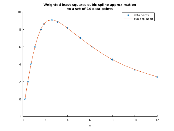
Determine a weighted least squares cubic spline approximation with five intervals (four interior knots) to a set of

14

given data points. Tabulate the data and the corresponding values of the approximating spline, together with the residual errors, and also the values of the approximating spline at points half-way between each pair of adjacent data points.

The example program is written in a general form that will enable a cubic spline approximation with

\bar{n}

intervals (

\bar{n} - 1

interior knots) to be obtained to

m

data points, with arbitrary positive weights, and the approximation to be tabulated. Note that nag_fit_1dspline_eval (e02bb) is used to evaluate the approximating spline. The program is self-starting in that any number of datasets can be supplied.

function e02ba_example


fprintf('e02ba example results\n\n');

m = 14;
data = [  0.20  0.00  0.2;
          0.47  2.00  0.2;
          0.74  4.00  0.3;
          1.09  6.00  0.7;
          1.60  8.00  0.9;
          1.90  8.62  1.0;
          2.60  9.10  1.0;
          3.10  8.90  1.0;
          4.00  8.15  0.8;
          5.15  7.00  0.5;
          6.17  6.00  0.7;
          8.00  4.54  1.0;
         10.00  3.39  1.0;
         12.00  2.56  1.0];
x = data(:,1);
y = data(:,2);
w = data(:,3);
     
knots = [1.5  2.6   4   8];
nbar  = size(knots,2) + 1;
ncap7 = nbar + 7;
lamda = zeros(ncap7,1);
lamda(5:nbar+3) = knots;

[lamda, c, ss, ifail] = e02ba( ...
                               x, y, w, lamda);

fprintf('\n  j       lamda(j+2)     b-spline coeff c(j)\n\n');
fprintf('%3d%35.4f\n', 1, c(1));
for j = 2:nbar+2
  fprintf('%3d%15.4f%20.4f\n',j,lamda(j+2),c(j));
end
fprintf('%3d%35.4f\n', nbar+3, c(nbar+3));
fprintf('\nResidual sum of squares = %12.2e\n\n', ss)
fprintf('Cubic spline approximation and residuals\n\n');
fprintf('       x          w          y         Fit     Residual\n');

k = 0;
for i = 1:m
  % data point evaluation
  k = k + 1;
  xp(k) = x(i);
  [fit(k), ifail] = e02bb( ...
                           lamda, c, x(i));
  fprintf('%11.4f%11.4f%11.4f%11.4f%11.2e\n', ...
          x(i), w(i), y(i), fit(k), fit(k)-y(i));
  % mid point evaluation
  if i<m
    xh = (x(i)+x(i+1))/2;
    k = k + 1;
    xp(k) = xh;
    [fit(k), ifail] = e02bb( ...
                             lamda, c, xh);
    fprintf('%11.4f%33.4f\n',xh, fit(k))
  end
end

fig1 = figure;
hold on
plot(x,y,'*')
plot(xp,fit);
xlabel('x');
title({'Weighted least-squares cubic spline approximation', ...
       'to a set of 14 data points'});
legend('data points','cubic spline fit');
hold off;

e02ba example results


  j       lamda(j+2)     b-spline coeff c(j)

  1                            -0.0465
  2         0.2000              3.6150
  3         1.5000              8.5724
  4         2.6000              9.4261
  5         4.0000              7.2716
  6         8.0000              4.1207
  7        12.0000              3.0822
  8                             2.5597

Residual sum of squares =     1.78e-03

Cubic spline approximation and residuals

       x          w          y         Fit     Residual
     0.2000     0.2000     0.0000    -0.0465  -4.65e-02
     0.3350                           1.0622
     0.4700     0.2000     2.0000     2.1057   1.06e-01
     0.6050                           3.0817
     0.7400     0.3000     4.0000     3.9880  -1.20e-02
     0.9150                           5.0558
     1.0900     0.7000     6.0000     5.9983  -1.73e-03
     1.3450                           7.1376
     1.6000     0.9000     8.0000     7.9872  -1.28e-02
     1.7500                           8.3544
     1.9000     1.0000     8.6200     8.6348   1.48e-02
     2.2500                           9.0076
     2.6000     1.0000     9.1000     9.0896  -1.04e-02
     2.8500                           9.0353
     3.1000     1.0000     8.9000     8.9125   1.25e-02
     3.5500                           8.5660
     4.0000     0.8000     8.1500     8.1321  -1.79e-02
     4.5750                           7.5592
     5.1500     0.5000     7.0000     6.9925  -7.53e-03
     5.6600                           6.5010
     6.1700     0.7000     6.0000     6.0255   2.55e-02
     7.0850                           5.2292
     8.0000     1.0000     4.5400     4.5315  -8.51e-03
     9.0000                           3.9045
    10.0000     1.0000     3.3900     3.3928   2.76e-03
    11.0000                           2.9574
    12.0000     1.0000     2.5600     2.5597  -3.45e-04

NAG Toolbox: nag_fit_1dspline_knots (e02ba)

▸▿ Contents

Purpose

Syntax

Description

References

Parameters

Compulsory Input Parameters

Optional Input Parameters

Output Parameters

Error Indicators and Warnings

Accuracy

Further Comments

Example

References

Cox M G (1972) The numerical evaluation of B-splines J. Inst. Math. Appl. 10 134–149
Cox M G (1974) A data-fitting package for the non-specialist user Software for Numerical Mathematics (ed D J Evans) Academic Press
Cox M G (1975) Numerical methods for the interpolation and approximation of data by spline functions PhD Thesis City University, London
Cox M G and Hayes J G (1973) Curve fitting: a guide and suite of algorithms for the non-specialist user NPL Report NAC26 National Physical Laboratory
de Boor C (1972) On calculating with B-splines J. Approx. Theory 6 50–62
Gentleman W M (1973) Least squares computations by Givens transformations without square roots J. Inst. Math. Applic. 12 329–336
Gentleman W M (1974) Algorithm AS 75. Basic procedures for large sparse or weighted linear least squares problems Appl. Statist. 23 448–454
Schoenberg I J and Whitney A (1953) On Polya frequency functions III Trans. Amer. Math. Soc. 74 246–259