NAG Toolbox: nag_ode_ivp_stiff_exp_bandjac (d02nc)

Purpose

Syntax

Description

.
.
.
[...] = d02nv(...);
[...] = d02nt(...);
[..., ifail] = d02nc(...);
if (ifail ~= 1 and ifail < 14) 
  [...] = d02ny(...);
end
.
.
.

References

Parameters

Compulsory Input Parameters

1:     $\mathrm{t}$ – double scalar

$t$, the value of the independent variable. The input value of t is used only on the first call as the initial point of the integration.

2:     $\mathrm{tout}$ – double scalar

The next value of $t$ at which a computed solution is desired. For the initial $t$, the input value of tout is used to determine the direction of integration. Integration is permitted in either direction (see also itask).

Constraint: $\mathbf{tout}\ne \mathbf{t}$.

3:     $\mathrm{y}\left(\mathbf{neq}\right)$ – double array

The values of the dependent variables (solution). On the first call the first neq elements of y must contain the vector of initial values.

4:     $\mathrm{rwork}\left(50+4\times \mathbf{neq}\right)$ – double array

5:     $\mathrm{rtol}\left(:\right)$ – double array

The dimension of the array rtol must be at least $1$ if $\mathbf{itol}=1$ or $2$, and at least $\mathbf{neq}$ otherwise

The relative local error tolerance.

Constraint: $\mathbf{rtol}\left(i\right)\ge 0.0$ for all relevant $i$ (see itol).

6:     $\mathrm{atol}\left(:\right)$ – double array

The dimension of the array atol must be at least $1$ if $\mathbf{itol}=1$ or $3$, and at least $\mathbf{neq}$ otherwise

The absolute local error tolerance.

Constraint: $\mathbf{atol}\left(i\right)\ge 0.0$ for all relevant $i$ (see itol).

7:     $\mathrm{itol}$ – int64int32nag_int scalar

A value to indicate the form of the local error test. itol indicates to nag_ode_ivp_stiff_exp_bandjac (d02nc) whether to interpret either or both of rtol or atol as a vector or a scalar. The error test to be satisfied is $‖e_i/w_i‖<1.0$, where $w_i$ is defined as follows:

itol	rtol	atol	$w_i$
1	scalar	scalar	$\mathbf{rtol}\left(1\right)\times \left|y_i\right|+\mathbf{atol}\left(1\right)$
2	scalar	vector	$\mathbf{rtol}\left(1\right)\times \left|y_i\right|+\mathbf{atol}\left(i\right)$
3	vector	scalar	$\mathbf{rtol}\left(i\right)\times \left|y_i\right|+\mathbf{atol}\left(1\right)$
4	vector	vector	$\mathbf{rtol}\left(i\right)\times \left|y_i\right|+\mathbf{atol}\left(i\right)$

$e_i$ is an estimate of the local error in $y_i$, computed internally, and the choice of norm to be used is defined by a previous call to an integrator setup function.

Constraint: $\mathbf{itol}=1$, $2$, $3$ or $4$.

8:     $\mathrm{inform}\left(23\right)$ – int64int32nag_int array

9:     $\mathrm{fcn}$ – function handle or string containing name of m-file

fcn must evaluate the derivative vector for the explicit ordinary differential equation system, defined by $y^{\prime }=g\left(t,y\right)$.

[f, ires] = fcn(neq, t, y, ires)

Input Parameters

1:     $\mathrm{neq}$ – int64int32nag_int scalar

The number of differential equations being solved.

2:     $\mathrm{t}$ – double scalar

$t$, the current value of the independent variable.

3:     $\mathrm{y}\left(\mathbf{neq}\right)$ – double array

The value of $y_{\mathit{i}}$, for $\mathit{i}=1,2,\dots ,\mathbf{neq}$.

4:     $\mathrm{ires}$ – int64int32nag_int scalar

$\mathbf{ires}=1$.

Output Parameters

1:     $\mathrm{f}\left(\mathbf{neq}\right)$ – double array

The value $y_{\mathit{i}}^{\prime }$, given by $y_{\mathit{i}}^{\prime }=g_{\mathit{i}}\left(t,y\right)$, for $\mathit{i}=1,2,\dots ,\mathbf{neq}$.

2:     $\mathrm{ires}$ – int64int32nag_int scalar

You may set ires as follows to indicate certain conditions in fcn to the integrator:

$\mathbf{ires}=1$

Indicates a normal return from fcn, that is ires has not been altered by you and integration continues.

$\mathbf{ires}=2$

Indicates to the integrator that control should be passed back immediately to the calling (sub)program with the error indicator set to $\mathbf{ifail}=\mathbf{11}$.

$\mathbf{ires}=3$

Indicates to the integrator that an error condition has occurred in the solution vector, its time derivative or in the value of $t$. The integrator will use a smaller time step to try to avoid this condition. If this is not possible the integrator returns to the calling (sub)program with the error indicator set to $\mathbf{ifail}=\mathbf{7}$.

$\mathbf{ires}=4$

Indicates to the integrator to stop its current operation and to enter monitr immediately with argument $\mathbf{imon}=-2$.

10:   $\mathrm{ysav}\left(\mathit{ldysav},\mathbf{sdysav}\right)$ – double array

ldysav, the first dimension of the array, must satisfy the constraint $\mathit{ldysav}\ge \mathbf{neq}$.

An appropriate value for sdysav is described in the specification of the integrator setup functions nag_ode_ivp_stiff_bdf (d02nv) and nag_ode_ivp_stiff_blend (d02nw). This value must be the same as that supplied to the integrator setup function.

11:   $\mathrm{jac}$ – function handle or string containing name of m-file

jac must evaluate the Jacobian of the system. If this option is not required, the actual argument for jac must be the string nag_ode_ivp_stiff_exp_bandjac_dummy_jac (d02ncz). (nag_ode_ivp_stiff_exp_bandjac_dummy_jac (d02ncz) is included in the NAG Toolbox.) You must indicate to the integrator whether this option is to be used by setting the argument jceval appropriately in a call to the banded linear algebra setup function nag_ode_ivp_stiff_bandjac_setup (d02nt).

First we must define the system of nonlinear equations which is solved internally by the integrator. The time derivative, $y^{\prime }$, generated internally, has the form

$$y^{\prime }=\left(y-z\right)/\left(hd\right)\text{,}$$

where $h$ is the current step size and $d$ is a argument that depends on the integration method in use. The vector $y$ is the current solution and the vector $z$ depends on information from previous time steps. This means that $\frac{d}{d{y}^{\prime }}\left(\text{ }\right)=\left(hd\right)\frac{d}{dy}\left(\text{ }\right)$. The system of nonlinear equations that is solved has the form

$$y^{\prime }-g\left(t,y\right)=0$$

but it is solved in the form

$$r\left(t,y\right)=0\text{,}$$

where $r$ is the function defined by

$$r\left(t,y\right)=\left(hd\right)\left(\left(y-z\right)/\left(hd\right)-g\left(t,y\right)\right)\text{.}$$

It is the Jacobian matrix $\frac{\partial r}{\partial y}$ that you must supply in jac as follows:

$$\begin{array}{ll}\frac{\partial r_i}{\partial y_j}=1-\left(hd\right)\frac{\partial g_i}{\partial y_j}\text{,}& \text{if }i=j\text{,}\\ & \\ \frac{\partial r_i}{\partial y_j}=-\left(hd\right)\frac{\partial g_i}{\partial y_j}\text{,}& \text{otherwise.}\end{array}$$

[p] = jac(neq, t, y, h, d, ml, mu, p)

Input Parameters

1:     $\mathrm{neq}$ – int64int32nag_int scalar

The number of differential equations being solved.

2:     $\mathrm{t}$ – double scalar

$t$, the current value of the independent variable.

3:     $\mathrm{y}\left(\mathbf{neq}\right)$ – double array

$y_{\mathit{i}}$, for $\mathit{i}=1,2,\dots ,\mathbf{neq}$, the current solution component.

4:     $\mathrm{h}$ – double scalar

The current step size.

5:     $\mathrm{d}$ – double scalar

The argument $d$ which depends on the integration method.

6:     $\mathrm{ml}$ – int64int32nag_int scalar

7:     $\mathrm{mu}$ – int64int32nag_int scalar

The number of subdiagonals and superdiagonals respectively in the band.

8:     $\mathrm{p}\left(\mathbf{ml}+\mathbf{mu}+1,\mathbf{neq}\right)$ – double array

Is set to zero.

Output Parameters

1:     $\mathrm{p}\left(\mathbf{ml}+\mathbf{mu}+1,\mathbf{neq}\right)$ – double array

Elements of the Jacobian matrix $\frac{\partial r}{\partial y}$ stored as specified by the following pseudocode:

 for i = 1:neq
 j1 = max(i-ml,1);
 j2 = min(i+mu,neq);
 for j = j1:j2
 k = min(ml+1-i,0)+j;
 p(k,i) = δr/δy(i,j);
 end
 end 

See also nag_lapack_dgbtrf (f07bd).

Only nonzero elements of this array need be set, since it is preset to zero before the call to jac.

12:   $\mathrm{wkjac}\left(\mathit{nwkjac}\right)$ – double array

nwkjac, the dimension of the array, must satisfy the constraint $\mathit{nwkjac}\ge \left(2m_L+m_U+1\right)\times \mathbf{neq}$, where $m_L$ and $m_U$ are the number of subdiagonals and superdiagonals respectively in the band, defined by a call to nag_ode_ivp_stiff_bandjac_setup (d02nt).

This value must be the same as that supplied to the linear algebra setup function nag_ode_ivp_stiff_bandjac_setup (d02nt).

Constraint: $\mathit{nwkjac}\ge \left(2m_L+m_U+1\right)\times \mathbf{neq}$, where $m_L$ and $m_U$ are the number of subdiagonals and superdiagonals respectively in the band, defined by a call to nag_ode_ivp_stiff_bandjac_setup (d02nt).

13:   $\mathrm{jacpvt}\left(\mathit{njcpvt}\right)$ – int64int32nag_int array

njcpvt, the dimension of the array, must satisfy the constraint $\mathit{njcpvt}\ge \mathit{ldysav}$.

This value must be the same as that supplied to the linear algebra setup function nag_ode_ivp_stiff_bandjac_setup (d02nt).

Constraint: $\mathit{njcpvt}\ge \mathit{ldysav}$.

14:   $\mathrm{monitr}$ – function handle or string containing name of m-file

monitr performs tasks requested by you. If this option is not required, then the actual argument for monitr must be the string nag_ode_ivp_stiff_exp_fulljac_dummy_monit (d02nby). (nag_ode_ivp_stiff_exp_fulljac_dummy_monit (d02nby) is included in the NAG Toolbox.)

[hnext, y, imon, inln, hmin, hmax] = monitr(neq, ldysav, t, hlast, hnext, y, ydot, ysav, r, acor, imon, hmin, hmax, nqu)

Input Parameters

1:     $\mathrm{neq}$ – int64int32nag_int scalar

The number of differential equations being solved.

2:     $\mathrm{ldysav}$ – int64int32nag_int scalar

An upper bound on the number of differential equations to be solved.

3:     $\mathrm{t}$ – double scalar

The current value of the independent variable.

4:     $\mathrm{hlast}$ – double scalar

The last step size successfully used by the integrator.

5:     $\mathrm{hnext}$ – double scalar

The step size that the integrator proposes to take on the next step.

6:     $\mathrm{y}\left(\mathbf{neq}\right)$ – double array

$y$, the values of the dependent variables evaluated at $t$.

7:     $\mathrm{ydot}\left(\mathbf{neq}\right)$ – double array

The time derivatives $y^{\prime }$ of the vector $y$.

8:     $\mathrm{ysav}\left(\mathit{ldysav},\mathit{sdysav}\right)$ – double array

Workspace to enable you to carry out interpolation using either of the functions nag_ode_ivp_stiff_nat_interp (d02xj) or nag_ode_ivp_stiff_c1_interp (d02xk).

9:     $\mathrm{r}\left(\mathbf{neq}\right)$ – double array

If $\mathbf{imon}=0$ and $\mathbf{inln}=3$, the first neq elements contain the residual vector, $y^{\prime }-g\left(t,y\right)$.

10:   $\mathrm{acor}\left(\mathbf{neq},2\right)$ – double array

With $\mathbf{imon}=1$, $\mathbf{acor}\left(i,1\right)$ contains the weight used for the $i$th equation when the norm is evaluated, and $\mathbf{acor}\left(i,2\right)$ contains the estimated local error for the $i$th equation. The scaled local error at the end of a timestep may be obtained by calling the double function nag_ode_ivp_stiff_errest (d02za) as follows:

 [errloc, ifail] = d02za(acor(1:neq,2), acor(1:neq,1));
 % Check ifail before proceeding 

11:   $\mathrm{imon}$ – int64int32nag_int scalar

A flag indicating under what circumstances monitr was called:

$\mathbf{imon}=-2$

Entry from the integrator after $\mathbf{ires}=4$ (set in fcn) caused an early termination (this facility could be used to locate discontinuities).

$\mathbf{imon}=-1$

The current step failed repeatedly.

$\mathbf{imon}=0$

Entry after a call to the internal nonlinear equation solver (see inln).

$\mathbf{imon}=1$

The current step was successful.

12:   $\mathrm{hmin}$ – double scalar

The minimum step size to be taken on the next step.

13:   $\mathrm{hmax}$ – double scalar

The maximum step size to be taken on the next step.

14:   $\mathrm{nqu}$ – int64int32nag_int scalar

The order of the integrator used on the last step. This is supplied to enable you to carry out interpolation using either of the functions nag_ode_ivp_stiff_nat_interp (d02xj) or nag_ode_ivp_stiff_c1_interp (d02xk).

Output Parameters

1:     $\mathrm{hnext}$ – double scalar

The next step size to be used. If this is different from the input value, then imon must be set to $4$.

2:     $\mathrm{y}\left(\mathbf{neq}\right)$ – double array

These values must not be changed unless imon is set to $2$.

3:     $\mathrm{imon}$ – int64int32nag_int scalar

May be reset to determine subsequent action in nag_ode_ivp_stiff_exp_bandjac (d02nc).

$\mathbf{imon}=-2$

Integration is to be halted. A return will be made from the integrator to the calling (sub)program with $\mathbf{ifail}=\mathbf{12}$.

$\mathbf{imon}=-1$

Allow the integrator to continue with its own internal strategy. The integrator will try up to three restarts unless imon is set $\ne -1$ on exit.

$\mathbf{imon}=0$

Return to the internal nonlinear equation solver, where the action taken is determined by the value of inln (see inln).

$\mathbf{imon}=1$

Normal exit to the integrator to continue integration.

$\mathbf{imon}=2$

Restart the integration at the current time point. The integrator will restart from order $1$ when this option is used. The solution y, provided by monitr, will be used for the initial conditions.

$\mathbf{imon}=3$

Try to continue with the same step size and order as was to be used before the call to monitr. hmin and hmax may be altered if desired.

$\mathbf{imon}=4$

Continue the integration but using a new value of hnext and possibly new values of hmin and hmax.

4:     $\mathrm{inln}$ – int64int32nag_int scalar

The action to be taken by the internal nonlinear equation solver when monitr is exited with $\mathbf{imon}=0$. By setting $\mathbf{inln}=3$ and returning to the integrator, the residual vector is evaluated and placed in the array r, and then monitr is called again. At present this is the only option available: inln must not be set to any other value.

5:     $\mathrm{hmin}$ – double scalar

The minimum step size to be used. If this is different from the input value, then imon must be set to $3$ or $4$.

6:     $\mathrm{hmax}$ – double scalar

The maximum step size to be used. If this is different from the input value, then imon must be set to $3$ or $4$. If hmax is set to zero, no limit is assumed.

15:   $\mathrm{itask}$ – int64int32nag_int scalar

The task to be performed by the integrator.

$\mathbf{itask}=1$

Normal computation of output values of $y\left(t\right)$ at $t=\mathbf{tout}$ (by overshooting and interpolating).

$\mathbf{itask}=2$

Take one step only and return.

$\mathbf{itask}=3$

Stop at the first internal integration point at or beyond $t=\mathbf{tout}$ and return.

$\mathbf{itask}=4$

Normal computation of output values of $y\left(t\right)$ at $t=\mathbf{tout}$ but without overshooting $t=\mathbf{tcrit}$. tcrit must be specified as an option in one of the integrator setup functions before the first call to the integrator, or specified in the optional input function before a continuation call. tcrit may be equal to or beyond tout, but not before it, in the direction of integration.

$\mathbf{itask}=5$

Take one step only and return, without passing tcrit. tcrit must be specified as under $\mathbf{itask}=4$.

Constraint: $\mathbf{itask}=1$, $2$, $3$, $4$ or $5$.

16:   $\mathrm{itrace}$ – int64int32nag_int scalar

The level of output that is printed by the integrator. itrace may take the value $-1$, $0$, $1$, $2$ or $3$.

$\mathbf{itrace}<-1$

$-1$ is assumed and similarly if $\mathbf{itrace}>3$, then $3$ is assumed.

$\mathbf{itrace}=-1$

No output is generated.

$\mathbf{itrace}=0$

Only warning messages are printed on the current error message unit (see nag_file_set_unit_error (x04aa)).

$\mathbf{itrace}>0$

Warning messages are printed as above, and on the current advisory message unit (see nag_file_set_unit_advisory (x04ab)) output is generated which details Jacobian entries, the nonlinear iteration and the time integration. The advisory messages are given in greater detail the larger the value of itrace.

Optional Input Parameters

1:     $\mathrm{neq}$ – int64int32nag_int scalar

Default: the dimension of the array y and the first dimension of the array ysav. (An error is raised if these dimensions are not equal.)

The number of differential equations to be solved.

Constraint: $\mathbf{neq}\ge 1$.

2:     $\mathrm{sdysav}$ – int64int32nag_int scalar

Default: the second dimension of the array ysav.

An appropriate value for sdysav is described in the specification of the integrator setup functions nag_ode_ivp_stiff_bdf (d02nv) and nag_ode_ivp_stiff_blend (d02nw). This value must be the same as that supplied to the integrator setup function.

Output Parameters

1:     $\mathrm{t}$ – double scalar

The value at which the computed solution $y$ is returned (usually at tout).

2:     $\mathrm{y}\left(\mathbf{neq}\right)$ – double array

The computed solution vector, evaluated at t (usually $\mathbf{t}=\mathbf{tout}$).

3:     $\mathrm{ydot}\left(\mathbf{neq}\right)$ – double array

The time derivatives $y^{\prime }$ of the vector $y$ at the last integration point.

4:     $\mathrm{rwork}\left(50+4\times \mathbf{neq}\right)$ – double array

5:     $\mathrm{inform}\left(23\right)$ – int64int32nag_int array

6:     $\mathrm{ysav}\left(\mathit{ldysav},\mathbf{sdysav}\right)$ – double array

Communication array, used to store information between calls to nag_ode_ivp_stiff_exp_bandjac (d02nc).

7:     $\mathrm{wkjac}\left(\mathit{nwkjac}\right)$ – double array

$\mathit{nwkjac}=\left(2m_L+m_U+1\right)\times \mathbf{neq}$, where $m_L$ and $m_U$ are the number of subdiagonals and superdiagonals respectively in the band, defined by a call to nag_ode_ivp_stiff_bandjac_setup (d02nt).

Communication array, used to store information between calls to nag_ode_ivp_stiff_exp_bandjac (d02nc).

8:     $\mathrm{jacpvt}\left(\mathit{njcpvt}\right)$ – int64int32nag_int array

$\mathit{njcpvt}=\mathit{ldysav}$.

Communication array, used to store information between calls to nag_ode_ivp_stiff_exp_bandjac (d02nc).

9:     $\mathrm{ifail}$ – int64int32nag_int scalar

$\mathbf{ifail}=\mathbf{0}$ unless the function detects an error (see Error Indicators and Warnings).

Error Indicators and Warnings

Cases prefixed with W are classified as warnings and do not generate an error of type NAG:error_n. See nag_issue_warnings.

   $\mathbf{ifail}=1$

An illegal input was detected on entry, or after an internal call to monitr. If $\mathbf{itrace}>-1$, then the form of the error will be detailed on the current error message unit (see nag_file_set_unit_error (x04aa)).

   $\mathbf{ifail}=2$

The maximum number of steps specified has been taken (see the description of optional inputs in the integrator setup functions and the optional input continuation function, nag_ode_ivp_stiff_contin (d02nz)).

   $\mathbf{ifail}=3$

With the given values of rtol and atol no further progress can be made across the integration range from the current point t. The components $\mathbf{y}\left(1\right),\mathbf{y}\left(2\right),\dots ,\mathbf{y}\left(\mathbf{neq}\right)$ contain the computed values of the solution at the current point t.

W  $\mathbf{ifail}=4$

There were repeated error test failures on an attempted step, before completing the requested task, but the integration was successful as far as t. The problem may have a singularity, or the local error requirements may be inappropriate.

W  $\mathbf{ifail}=5$

There were repeated convergence test failures on an attempted step, before completing the requested task, but the integration was successful as far as t. This may be caused by an inaccurate Jacobian matrix or one which is incorrectly computed.

W  $\mathbf{ifail}=6$

Some error weight $w_i$ became zero during the integration (see the description of itol). Pure relative error control ($\mathbf{atol}\left(i\right)=0.0$) was requested on a variable (the $i$th) which has now vanished. The integration was successful as far as t.

   $\mathbf{ifail}=7$

fcn set its error flag ($\mathbf{ires}=3$) continually despite repeated attempts by the integrator to avoid this.

   $\mathbf{ifail}=8$

Not used for this integrator.

   $\mathbf{ifail}=9$

A singular Jacobian $\frac{\partial r}{\partial y}$ has been encountered. This error exit is unlikely to be taken when solving explicit ordinary differential equations. You should check the problem formulation and Jacobian calculation.

   $\mathbf{ifail}=10$

An error occurred during Jacobian formulation or back-substitution (a more detailed error description may be directed to the current error message unit, see nag_file_set_unit_error (x04aa)).

W  $\mathbf{ifail}=11$

fcn signalled the integrator to halt the integration and return ($\mathbf{ires}=2$). Integration was successful as far as t.

W  $\mathbf{ifail}=12$

monitr set $\mathbf{imon}=-2$ and so forced a return but the integration was successful as far as t.

W  $\mathbf{ifail}=13$

The requested task has been completed, but it is estimated that a small change in rtol and atol is unlikely to produce any change in the computed solution. (Only applies when you are not operating in one step mode, that is when $\mathbf{itask}\ne 2$ or $5$.)

   $\mathbf{ifail}=14$

The values of rtol and atol are so small that nag_ode_ivp_stiff_exp_bandjac (d02nc) is unable to start the integration.

   $\mathbf{ifail}=15$

The linear algebra setup function nag_ode_ivp_stiff_bandjac_setup (d02nt) was not called prior to calling nag_ode_ivp_stiff_exp_bandjac (d02nc).

   $\mathbf{ifail}=-99$

An unexpected error has been triggered by this routine. Please contact NAG.

   $\mathbf{ifail}=-399$

Your licence key may have expired or may not have been installed correctly.

   $\mathbf{ifail}=-999$

Dynamic memory allocation failed.

Accuracy

Further Comments

Example

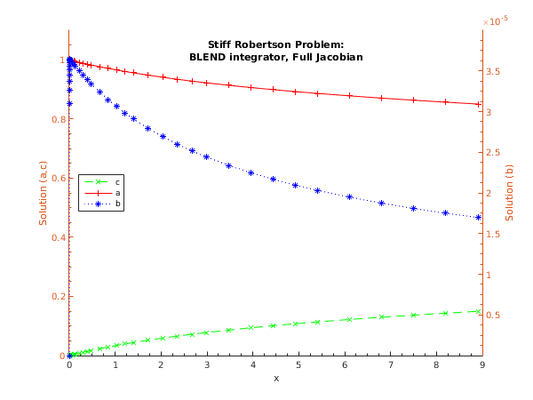
Open in the MATLAB editor: d02nc_example

function d02nc_example


fprintf('d02nc example results\n\n');

% For communication with monitr.
global ncall ykeep tkeep

% Initialize setup variables and arrays.
neq    = int64(3);
neqmax = int64(neq);
ml     = int64(1);
mu     = int64(2);
nwkjac = int64(neqmax*(2*ml+mu+1));
njcpvt = int64(neqmax);
maxord = int64(11);
sdysav = int64(maxord+3);
maxstp = int64(200);
mxhnil = int64(5);

h0    = 0;
hmax  = 10;
hmin  = 1.0e-10;
tcrit = 0;
petzld = false;

const  = zeros(6, 1);
rwork  = zeros(50+4*neqmax, 1);

% d02nw is a setup routine to be called prior to d02nc.
[const, rwork, ifail] = d02nw(...
                              neqmax, sdysav, maxord, const, tcrit, hmin, ...
                              hmax, h0, maxstp, mxhnil, 'Average-L2', rwork);

% d02nt is a setup routine to be called prior to d02nc.
[rwork, ifail] = d02nt(...
                       neq, neqmax, 'Analytic', ml, mu, nwkjac, njcpvt, rwork);


% Initialize integration variables and arrays.
inform(1:32) = int64(0);
ysave  = zeros(neq, sdysav);
wkjac  = zeros(nwkjac, 1);
jacpvt(1:njcpvt) = int64(0);

% First part.  Integrate to tout = 5.0 with itask=1 (i.e. overshooting and
% internal interpolation) using the blend method. 
% Employ scalar relative tolerance and a vector of absolute tolerances.
t      = 0.0;
tout   = 5.0;
itask  = int64(1);
itrace = int64(0);
y      = [1; 0; 0];
itol   = int64(2);
rtol   = [0.0001];
atol   = [1e-07; 1e-08; 1e-07];

% Prepare to store results for plotting.  This gets done in monitr.
ncall = 1;
tkeep(1) = t;
ykeep(1:3,1) = y(1:3);

% Output initial results.
fprintf('    x            y_1           y_2           y_3\n');
fprintf('%8.3f       %8.5f      %8.5f      %8.5f\n', t, y);

% The Jacobian is evaluated by jac, and a monitoring routine is provided.
[t, y, ydot, rwork, inform, ysave, wkjac, jacpvt, ifail] = ...
    d02nc(t, tout, y, rwork, rtol, atol, itol, inform, @fcn, ysave, @jac, ...
          wkjac, jacpvt, @monitr, itask, itrace);

% Output results.
fprintf('%8.3f       %8.5f      %8.5f      %8.5f\n', t, y);

% Seconnd part: continue integration to tout = 10.0 with  different stepsize.
h = 0.7;
[rwork, ifail] = d02nz(neqmax, tcrit, h, hmin, hmax, maxstp, mxhnil, rwork);

% Set tout and call integration routine.
tout = 10;
[t, y, ydot, rwork, inform, ysave, wkjac, jacpvt, ifail] = ...
  d02nc(t, tout, y, rwork, rtol, atol, itol, inform, @fcn, ysave, @jac, ...
        wkjac, jacpvt, @monitr, itask, itrace);

% Output results.
fprintf('%8.3f       %8.5f      %8.5f      %8.5f\n', t, y);

% d02ny is an integrator diagnostic routine which can be called after d02nc.
[hu, h, tcur, tolsf, nst, nre, nje, nqu, nq, niter, imxer, algequ, ...
    ifail] = d02ny(neq, neqmax, rwork, inform);

% Output diagnostics.
fprintf('\nDiagnostic information\n integration status:\n');
fprintf('   last and next step sizes = %8.5f, %8.5f\n',hu, h);
fprintf('   integration stopped at x = %8.5f\n',tcur);
fprintf(' algorithm statistics:\n');
fprintf('   number of time-steps and Newton iterations  = %5d %5d\n',nst,niter);
fprintf('   number of residual and jacobian evaluations = %5d %5d\n',nre,nje);
fprintf('   order of method last used and next to use   = %5d %5d\n',nqu,nq);
fprintf('   component with largest error                = %5d\n\n',imxer);
% Plot results.
fig1 = figure;
display_plot(tkeep(1:ncall),ykeep(1:3,1:ncall));


function [f, ires] = fcn(neq, t, y, ires)
% Evaluate derivative vector.
f = zeros(3,1);
f(1) = -0.04d0*y(1) + 1.0d4*y(2)*y(3);
f(2) = 0.04d0*y(1) - 1.0d4*y(2)*y(3) - 3.0d7*y(2)*y(2);
f(3) = 3.0d7*y(2)*y(2);

function p = jac(neq, t, y, h, d, ml, mu, pIn)
% Evaluate the Jacobian.
p = zeros(ml+mu+1, neq);
hxd = h*d;
p(1,1) = -hxd*(-0.04d0) + 1;
p(2,1) = -hxd*(1.0d4*y(3));
p(3,1) = -hxd*(1.0d4*y(2));
p(1,2) = -hxd*(0.04d0);
p(2,2) = -hxd*(-1.0d4*y(3)-6.0d7*y(2)) + 1;
p(3,2) = -hxd*(-1.0d4*y(2));
p(1,3) = -hxd*(6.0d7*y(2));
p(2,3) = -hxd*(0.0d0) + 1;

function [hnext, y, imon, inln, hmin, hmax] = monitr(neq, neqmax, ...
    t, hlast, hnext, y, ydot, ysave, r, acor, imon, hmin, hmax, nqu)
% For communication with main routine.
global ncall tkeep ykeep
% This example of a monitoring routine stores the current results if the
% integration step was successful, and if the x value is in range.
tend = 10.0;
if (imon == 1 && t>0.001 && t<tend)
    ncall = ncall + 1;
    tkeep(ncall) = t;
    ykeep(1:3,ncall) = y(1:3);
end
% We have to assign a value to inln (whether it gets used or not).
inln = int64(0);

function display_plot(tkeep,ykeep)
% Plot one of the curves and then add the other two.

hline3 = plot(tkeep,ykeep(3,:));
hold on;
[haxes, hline1, hline2] = plotyy(tkeep,ykeep(1,:), tkeep,ykeep(2,:));
% Set the axis limits and the tick specifications to beautify the plot.
set(haxes(1), 'YLim', [0.0 1.1]);
set(haxes(1), 'XMinorTick', 'on', 'YMinorTick', 'on');
set(haxes(1), 'YTick', [0.0 0.2 0.4 0.6 0.8 1.0]);
set(haxes(2), 'YLim', [0.0 4e-5]);
set(haxes(2), 'YMinorTick', 'on');
set(haxes(2), 'YTick', [0.5e-5:0.5e-5:3.5e-5]);
set(haxes(1), 'XLim', [0 9]);
set(haxes(2), 'XLim', [0 9]);
set(gca, 'box', 'off'); % no ticks on opposite axes.
% Add title.
ht = title({'Stiff Robertson Problem:','BLEND integrator, Full Jacobian'});
set(ht,'Position',[4.5,0.99,0.0]);
% Label the x axis, and both y axes.
xlabel('x');
ylabel(haxes(1),'Solution (a,c)');
ylabel(haxes(2),'Solution (b)');
% Add a legend.
legend('c','a','b','Location','West');
% Set some features of the lines.
set(hline1, 'Marker', '+','Linestyle','-','Color','red');
set(hline2, 'Marker', '*','Linestyle',':','Color','blue');
set(hline3, 'Marker', 'x','Linestyle','--','Color','green');
hold off;

d02nc example results

    x            y_1           y_2           y_3
   0.000        1.00000       0.00000       0.00000
   5.000        0.89152       0.00002       0.10846
  10.000        0.84137       0.00002       0.15861

Diagnostic information
 integration status:
   last and next step sizes =  1.12797,  1.12797
   integration stopped at x = 10.03368
 algorithm statistics:
   number of time-steps and Newton iterations  =    63   272
   number of residual and jacobian evaluations =   274    14
   order of method last used and next to use   =     4     4
   component with largest error                =     3