PDF version (NAG web site
, 64-bit version, 64-bit version)
NAG Toolbox: nag_tsa_cp_pelt_user (g13nb)
Purpose
nag_tsa_cp_pelt_user (g13nb) detects change points in a univariate time series, that is, the time points at which some feature of the data, for example the mean, changes. Change points are detected using the PELT (Pruned Exact Linear Time) algorithm using one of a provided set of cost function.
Syntax
Description
Let denote a series of data and denote a set of ordered (strictly monotonic increasing) indices known as change points with and . For ease of notation we also define . The change points, , split the data into segments, with the th segment being of length and containing .
Given a user-supplied cost function,
nag_tsa_cp_pelt_user (g13nb) solves
where
is a penalty term used to control the number of change points. This minimization is performed using the PELT algorithm of
Killick et al. (2012). The PELT algorithm is guaranteed to return the optimal solution to
(1) if there exists a constant
such that
for all
References
Chen J and Gupta A K (2010) Parametric Statistical Change Point Analysis With Applications to Genetics Medicine and Finance Second Edition Birkhäuser
Killick R, Fearnhead P and Eckely I A (2012) Optimal detection of changepoints with a linear computational cost Journal of the American Statistical Association 107:500 1590–1598
Parameters
Compulsory Input Parameters
- 1:
– int64int32nag_int scalar
-
, the length of the time series.
Constraint:
.
- 2:
– double scalar
-
, the penalty term.
There are a number of standard ways of setting
, including:
- SIC or BIC
-
- AIC
-
- Hannan-Quinn
-
where
is the number of parameters being treated as estimated in each segment. The value of
will depend on the cost function being used.
If no penalty is required then set . Generally, the smaller the value of the larger the number of suggested change points.
- 3:
– double scalar
-
, the constant value that satisfies equation
(2). If
exists, it is unlikely to be unique in such cases, it is recommened that the largest value of
, that satisfies equation
(2), is chosen. No check is made that
is the correct value for the supplied cost function.
- 4:
– function handle or string containing name of m-file
-
The cost function,
.
costfn must calculate a vector of costs for a number of segments.
[c, user, info] = costfn(ts, r, user, info)
Input Parameters
- 1:
– int64int32nag_int scalar
-
A reference time point.
- 2:
– int64int32nag_int array
-
Time points which, along with
ts, define the segments being considered,
for
.
- 3:
– Any MATLAB object
costfn is called from
nag_tsa_cp_pelt_user (g13nb) with the object supplied to
nag_tsa_cp_pelt_user (g13nb).
- 4:
– int64int32nag_int scalar
-
.
Output Parameters
- 1:
– double array
-
The cost function,
, with
where
and
.
It should be noted that if
for any value of
then it will be true for all values of
. Therefore the inequality need only be tested once per call to
costfn.
- 2:
– Any MATLAB object
- 3:
– int64int32nag_int scalar
-
Set
info to a nonzero value if you wish
nag_tsa_cp_pelt_user (g13nb) to terminate with
.
Optional Input Parameters
- 1:
– int64int32nag_int scalar
Default:
The minimum distance between two change points, that is .
Constraint:
.
- 2:
– Any MATLAB object
user is not used by
nag_tsa_cp_pelt_user (g13nb), but is passed to
costfn. Note that for large objects it may be more efficient to use a global variable which is accessible from the m-files than to use
user.
Output Parameters
- 1:
– int64int32nag_int array
-
The dimension of the array
tau will be
The location of the change points. The th segment is defined by to , where and .
- 2:
– Any MATLAB object
- 3:
– int64int32nag_int scalar
unless the function detects an error (see
Error Indicators and Warnings).
Error Indicators and Warnings
Errors or warnings detected by the function:
-
-
Constraint: .
-
-
Constraint: .
-
-
User requested termination.
-
An unexpected error has been triggered by this routine. Please
contact
NAG.
-
Your licence key may have expired or may not have been installed correctly.
-
Dynamic memory allocation failed.
Accuracy
Not applicable.
Further Comments
nag_tsa_cp_pelt (g13na) performs the same calculations for a cost function selected from a provided set of cost functions. If the required cost function belongs to this provided set then
nag_tsa_cp_pelt (g13na) can be used without the need to provide a cost function routine.
Example
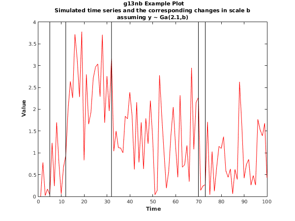
This example identifies changes in the scale parameter, under the assumption that the data has a gamma distribution, for a simulated dataset with observations. A penalty, of is used and the minimum segment size is set to . The shape parameter is fixed at across the whole input series.
The cost function used is
where
is a shape parameter that is fixed for all segments and
.
Open in the MATLAB editor:
g13nb_example
function g13nb_example
fprintf('g13nb example results\n\n');
y = [ 0.00; 0.78; 0.02; 0.17; 0.04; 1.23; 0.24; 1.70; 0.77; 0.06;
0.67; 0.94; 1.99; 2.64; 2.26; 3.72; 3.14; 2.28; 3.78; 0.83;
2.80; 1.66; 1.93; 2.71; 2.97; 3.04; 2.29; 3.71; 1.69; 2.76;
1.96; 3.17; 1.04; 1.50; 1.12; 1.11; 1.00; 1.84; 1.78; 2.39;
1.85; 0.62; 2.16; 0.78; 1.70; 0.63; 1.79; 1.21; 2.20; 1.34;
0.04; 0.14; 2.78; 1.83; 0.98; 0.19; 0.57; 1.41; 2.05; 1.17;
0.44; 2.32; 0.67; 0.73; 1.17; 0.34; 2.95; 1.08; 2.16; 2.27;
0.14; 0.24; 0.27; 1.71; 0.04; 1.03; 0.12; 0.67; 1.15; 1.10;
1.37; 0.59; 0.44; 0.63; 0.06; 0.62; 0.39; 2.63; 1.63; 0.42;
0.73; 0.85; 0.26; 0.48; 0.26; 1.77; 1.53; 1.39; 1.68; 0.43];
csy = [0.0; cumsum(y)];
a = 2.1;
k = 0;
user = {csy; a};
n = int64(numel(y));
beta = 3.4;
minss = int64(3);
[tau] = g13nb( ...
n, beta, k, @costfn, 'minss', minss, 'user', user);
fprintf(' -- Change Points --\n');
fprintf(' Number Position\n');
fprintf(' =====================\n');
for i = 1:numel(tau)
fprintf(' %4d %6d\n', i, tau(i));
end
fig1 = figure;
plot(y,'Color','red');
xpos = transpose(double(tau(1:end-1))*ones(1,2));
ypos = diag(ylim)*ones(2,numel(tau)-1);
line(xpos,ypos,'Color','black');
title({'{\bf g13nb Example Plot}',
'Simulated time series and the corresponding changes in scale b',
'assuming y ~ Ga(2.1,b)'});
xlabel('{\bf Time}');
ylabel('{\bf Value}');
function [c,user,info] = costfn(ts, r, user, info)
csy = user{1};
a = user{2};
if (ts<r(1))
si = csy(r+1) - csy(ts+1);
dn = double(r - ts);
else
si = csy(ts+1) - csy(r+1);
dn = double(ts - r);
end
c = (2*dn*a) .* (log(si) - log(dn*a));
info = int64(0);
g13nb example results

  -- Change Points --
  Number     Position
 =====================
    1            5
    2           12
    3           32
    4           70
    5           73
    6          100
This example plot shows the original data series and the estimated change points.
PDF version (NAG web site
, 64-bit version, 64-bit version)
© The Numerical Algorithms Group Ltd, Oxford, UK. 2009–2015
