PDF version (NAG web site
, 64-bit version, 64-bit version)
NAG Toolbox: nag_fit_2dspline_evalv (e02de)
Purpose
nag_fit_2dspline_evalv (e02de) calculates values of a bicubic spline from its B-spline representation.
Syntax
[
ff,
ifail] = e02de(
x,
y,
lamda,
mu,
c, 'm',
m, 'px',
px, 'py',
py)
[
ff,
ifail] = nag_fit_2dspline_evalv(
x,
y,
lamda,
mu,
c, 'm',
m, 'px',
px, 'py',
py)
Description
nag_fit_2dspline_evalv (e02de) calculates values of the bicubic spline
at prescribed points
, for
, from its augmented knot sets
and
and from the coefficients
, for
and
, in its B-spline representation
Here
and
denote normalized cubic B-splines, the former defined on the knots
to
and the latter on the knots
to
.
This function may be used to calculate values of a bicubic spline given in the form produced by
nag_interp_2d_spline_grid (e01da),
nag_fit_2dspline_panel (e02da),
nag_fit_2dspline_grid (e02dc) and
nag_fit_2dspline_sctr (e02dd). It is derived from the function B2VRE in
Anthony et al. (1982).
References
Anthony G T, Cox M G and Hayes J G (1982) DASL – Data Approximation Subroutine Library National Physical Laboratory
Cox M G (1978) The numerical evaluation of a spline from its B-spline representation J. Inst. Math. Appl. 21 135–143
Parameters
Compulsory Input Parameters
- 1:
– double array
- 2:
– double array
-
x and
y must contain
and
, for
, respectively. These are the coordinates of the points at which values of the spline are required. The order of the points is immaterial.
Constraint:
and
must satisfy
and
.
The spline representation is not valid outside these intervals.
- 3:
– double array
- 4:
– double array
-
lamda and
mu must contain the complete sets of knots
and
associated with the
and
variables respectively.
Constraint:
the knots in each set must be in nondecreasing order, with and .
- 5:
– double array
-
must contain the coefficient
described in
Description, for
and
.
Optional Input Parameters
- 1:
– int64int32nag_int scalar
-
Default:
the dimension of the arrays
x,
y. (An error is raised if these dimensions are not equal.)
, the number of points at which values of the spline are required.
Constraint:
.
- 2:
– int64int32nag_int scalar
- 3:
– int64int32nag_int scalar
-
Default:
For
px, the dimension of the array
lamda. For
py, the dimension of the array
mu.
px and
py must specify the total number of knots associated with the variables
and
respectively. They are such that
and
are the corresponding numbers of interior knots.
Constraint:
and .
Output Parameters
- 1:
– double array
-
contains the value of the spline at the point , for .
- 2:
– int64int32nag_int scalar
unless the function detects an error (see
Error Indicators and Warnings).
Error Indicators and Warnings
Errors or warnings detected by the function:
-
-
| On entry, | , |
| or | , |
| or | . |
-
-
On entry, the knots in array
lamda, or those in array
mu, are not in nondecreasing order, or
, or
.
-
-
On entry, at least one of the prescribed points lies outside the rectangle defined by , and , .
-
An unexpected error has been triggered by this routine. Please
contact
NAG.
-
Your licence key may have expired or may not have been installed correctly.
-
Dynamic memory allocation failed.
Accuracy
The method used to evaluate the B-splines is numerically stable, in the sense that each computed value of
can be regarded as the value that would have been obtained in exact arithmetic from slightly perturbed B-spline coefficients. See
Cox (1978) for details.
Further Comments
Computation time is approximately proportional to the number of points, , at which the evaluation is required.
Example
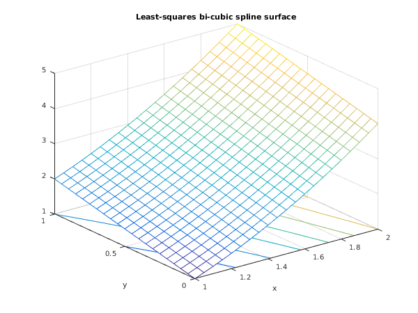
This program reads in knot sets and , and a set of bicubic spline coefficients . Following these are a value for and the coordinates , for , at which the spline is to be evaluated.
Open in the MATLAB editor:
e02de_example
function e02de_example
fprintf('e02de example results\n\n');
lamda = [1 1 1 1 1.3 1.5 1.6 2 2 2 2];
mu = [0 0 0 0 0.4 0.7 1 1 1 1];
c = [1 1.2 1.5833 2.1433 2.8667 3.4667 4;
1.1333 1.3333 1.7167 2.2767 3 3.6 4.1333;
1.3667 1.5667 1.95 2.51 3.2333 3.8333 4.3667;
1.7 1.9 2.2833 2.8433 3.5667 4.1667 4.7;
1.9 2.1 2.4833 3.0433 3.7667 4.3667 4.9;
2 2.2 2.5833 3.1433 3.8667 4.4667 5];
x = [1 1.1 1.5 1.6 1.9 1.9 2];
y = [0 0.1 0.7 0.4 0.3 0.8 1];
[ff, ifail] = e02de( ...
x, y, lamda, mu, c);
fprintf(' x y fit\n');
fprintf('%11.3f%11.3f%11.3f\n',[x; y; ff']);
mx = [1:0.05:2];
my = [0:0.05:1];
for i = 1:21
xx(1:21) = mx(i);
[ff(1:21,i), ifail] = e02de( ...
xx, my, lamda, mu, c);
end
fig1 = figure;
meshc(mx,my,ff);
xlabel('x');
ylabel('y');
title('Least-squares bi-cubic spline surface');
e02de example results

        x          y          fit
      1.000      0.000      1.000
      1.100      0.100      1.310
      1.500      0.700      2.950
      1.600      0.400      2.960
      1.900      0.300      3.910
      1.900      0.800      4.410
      2.000      1.000      5.000
PDF version (NAG web site
, 64-bit version, 64-bit version)
© The Numerical Algorithms Group Ltd, Oxford, UK. 2009–2015
