d03px:: Partial Differential Equations (NAG Toolbox)

nag_pde_1d_parab_euler_exact (d03px) calculates a numerical flux function at a single spatial point using an Exact Riemann Solver (see Toro (1996) and Toro (1989)) for the Euler equations (for a perfect gas) in conservative form. You must supply the left and right solution values at the point where the numerical flux is required, i.e., the initial left and right states of the Riemann problem defined below. In nag_pde_1d_parab_convdiff (d03pf), nag_pde_1d_parab_convdiff_dae (d03pl) and nag_pde_1d_parab_convdiff_remesh (d03ps), the left and right solution values are derived automatically from the solution values at adjacent spatial points and supplied to the function argument numflx from which you may call nag_pde_1d_parab_euler_exact (d03px).

The function calculates the numerical flux function

F (U_{L}, U_{R}) = F (U^{*} (U_{L}, U_{R}))

, where

U = U_{L}

and

U = U_{R}

are the left and right solution values, and

U^{*} (U_{L}, U_{R})

is the intermediate state

ω (0)

arising from the similarity solution

U (y, t) = ω (y / t)

of the Riemann problem defined by

\frac{\partial U}{\partial t} + \frac{\partial F}{\partial y} = 0,

(4)

with

U

and

F

as in (2), and initial piecewise constant values

U = U_{L}

for

y < 0

and

U = U_{R}

for

y > 0

. The spatial domain is

- \infty < y < \infty

, where

y = 0

is the point at which the numerical flux is required.

References

Parameters

Compulsory Input Parameters

Optional Input Parameters

Output Parameters

Error Indicators and Warnings

Accuracy

Further Comments

Example

This example uses nag_pde_1d_parab_convdiff_dae (d03pl) and nag_pde_1d_parab_euler_exact (d03px) to solve the Euler equations in the domain

0 \leq x \leq 1

for

0 < t \leq 0.035

with initial conditions for the primitive variables

ρ (x, t)

u (x, t)

and

p (x, t)

given by

\begin{array}{llcrlcrl} ρ (x, 0) = 5.99924, & u (x, 0) = 19.5975, & p (x, 0) = 460.894, & for ​ x < 0.5, \\ ρ (x, 0) = 5.99242, & u (x, 0) = - 6.19633, & p (x, 0) = 46.095, & for ​ x > 0.5 . \end{array}

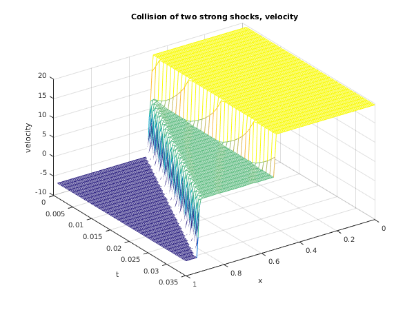
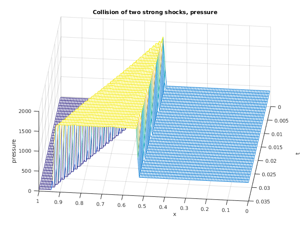
This test problem is taken from Toro (1996) and its solution represents the collision of two strong shocks travelling in opposite directions, consisting of a left facing shock (travelling slowly to the right), a right travelling contact discontinuity and a right travelling shock wave. There is an exact solution to this problem (see Toro (1996)) but the calculation is lengthy and has therefore been omitted.

function d03px_example


fprintf('d03px example results\n\n');

global gamma rl0 rr0 ul0 ur0 el0 er0;

% Problem parameters
alpha_l = 460.894;
alpha_r = 46.095;
beta_l  = 19.5975;
beta_r  =  6.19633;
gamma  =   1.4;
rl0    =   5.99924;
rr0    =   5.99242;
ul0    = 117.5701059;
ur0    = -37.1310118186;
el0    = alpha_l/(gamma-1) + rl0*beta_l^2/2;
er0    = alpha_r/(gamma-1) + rr0*beta_r^2/2;

npde  = int64(3);
npts  = int64(141);
ncode = int64(0);
nxi   = int64(0);
neqn  = npde*npts+ncode;
ts    = 0;
xi    = [];
itol = int64(1);
atol = [0.005];
rtol = [0.0005];
norm_p = '2';
laopt = 'B';
algopt = zeros(30,1);
algopt(1) = 2;
algopt(6) = 2;
algopt(7) = 2;
algopt(13) = 0.005;
rsave  = zeros(21000, 1);
isave  = zeros(25700, 1, 'int64');
itask  = int64(1);
itrace = int64(0);
ind    = int64(0);

% Initial mesh and solution
dx = 1/(double(npts)-1);
x  = [0:dx:1];
u = uvinit(x);

u1sol = zeros(35,npts);
u2sol = zeros(35,npts);
u3sol = zeros(35,npts);
xsol = zeros(35,npts);
tsol = zeros(35,npts);

for j=1:35
  tout = 0.001*j;
  [ts, u, rsave, isave, ind, ifail] = ...
  d03pl( ...
         npde, ts, tout, 'd03plp', @numflx, @bndary, u, x, ncode, ...
         'd03pek', xi, rtol, atol, itol, norm_p, laopt, ...
         algopt, rsave, isave, itask, itrace, ind,'nxi',nxi);

  xsol(j,:) = x;
  tsol(j,:) = ts;
  u1sol(j,:) = u(1,:);
  u2sol(j,:) = u(2,:)./u(1,:);
  u3sol(j,:) = 0.4*u(1,:).*(u(3,:)./u(1,:)-u2sol(j,:).^2/2);
  
end

nsteps = 50*((isave(1)+25)/50);
nfuncs = 50*((isave(2)+25)/50);
njacs = isave(3);
niters = isave(5);
fprintf('\n Number of time steps           (nearest 50) = %6d\n',nsteps);
fprintf(' Number of function evaluations (nearest 50) = %6d\n',nfuncs);
fprintf(' Number of Jacobian evaluations (nearest  1) = %6d\n',njacs);
fprintf(' Number of iterations           (nearest  1) = %6d\n',niters);

fig1=figure;
mesh(xsol,tsol,u1sol);
title('Collision of two strong shocks, density');
xlabel('x');
ylabel('t');
zlabel('density');
view(182,40);

fig2=figure;
mesh(xsol,tsol,u2sol);
title('Collision of two strong shocks, velocity');
xlabel('x');
ylabel('t');
zlabel('velocity');
view(145,40);

fig3=figure;
mesh(xsol,tsol,u3sol);
title('Collision of two strong shocks, pressure');
xlabel('x');
ylabel('t');
zlabel('pressure');
view(-174,50);



function [g, iresout] = bndary(npde, npts, t, x, u, ncode, ...
                               v, vdot, ibnd, ires)
  
  global rl0 rr0 ul0 ur0 el0 er0;

  if (ibnd == 0)
    g(1) = u(1,1) - rl0;
    g(2) = u(2,1) - ul0;
    g(3) = u(3,1) - el0;
  else
    g(1) = u(1,npts) - rr0;
    g(2) = u(2,npts) - ur0;
    g(3) = u(3,npts) - er0;
  end
  iresout = ires;

function [flux, ires] = numflx(npde, t, x, ncode, v, uleft, uright, ires)

  global gamma;

  % Exact Reimann solver.

  tol = 0;
  niter  = int64(0);
  [flux, ifail] = d03px( ...
                         uleft, uright, gamma, tol, niter);

function [u] = uvinit(x)

  global rl0 rr0 ul0 ur0 el0 er0;

  n = size(x,2);
  u = zeros(3,n);
  for i = 1:n
    if x(i)<1/2
      u(1,i) = rl0;
      u(2,i) = ul0;
      u(3,i) = el0;
    elseif x(i)== 1/2
      u(1,i) = (rl0+rr0)/2;
      u(2,i) = (ul0+ur0)/2;
      u(3,i) = (el0+er0)/2;
    else
      u(1,i) = rr0;
      u(2,i) = ur0;
      u(3,i) = er0;
    end
  end

On entry,	$gamma \leq 0.0$ ,
or	$tol < 0.0$ ,
or	$niter < 0$ .

NAG Toolbox: nag_pde_1d_parab_euler_exact (d03px)

▸▿ Contents

Purpose

Syntax

Description