PDF version (NAG web site
, 64-bit version, 64-bit version)
NAG Toolbox: nag_smooth_fit_spline (g10ab)
Purpose
nag_smooth_fit_spline (g10ab) fits a cubic smoothing spline for a given smoothing parameter.
Syntax
[
yhat,
c,
rss,
df,
res,
h,
comm,
ifail] = g10ab(
mode,
x,
y,
rho,
c,
comm, 'n',
n, 'wt',
wt)
[
yhat,
c,
rss,
df,
res,
h,
comm,
ifail] = nag_smooth_fit_spline(
mode,
x,
y,
rho,
c,
comm, 'n',
n, 'wt',
wt)
Note: the interface to this routine has changed since earlier releases of the toolbox:
| At Mark 24: |
weight was removed from the interface; wt was made optional |
Description
nag_smooth_fit_spline (g10ab) fits a cubic smoothing spline to a set of observations (, ), for . The spline provides a flexible smooth function for situations in which a simple polynomial or nonlinear regression model is unsuitable.
Cubic smoothing splines arise as the unique real-valued solution function
, with absolutely continuous first derivative and squared-integrable second derivative, which minimizes:
where
is the (optional) weight for the
th observation and
is the smoothing parameter. This criterion consists of two parts: the first measures the fit of the curve, and the second the smoothness of the curve. The value of the smoothing parameter
weights these two aspects; larger values of
give a smoother fitted curve but, in general, a poorer fit. For details of how the cubic spline can be estimated see
Hutchinson and de Hoog (1985) and
Reinsch (1967).
The fitted values,
, and weighted residuals,
, can be written as
for a matrix
. The residual degrees of freedom for the spline is
and the diagonal elements of
,
, are the leverages.
The parameter
can be chosen in a number of ways. The fit can be inspected for a number of different values of
. Alternatively the degrees of freedom for the spline, which determines the value of
, can be specified, or the (generalized) cross-validation can be minimized to give
; see
nag_smooth_fit_spline_parest (g10ac) for further details.
nag_smooth_fit_spline (g10ab) requires the
to be strictly increasing. If two or more observations have the same
-value then they should be replaced by a single observation with
equal to the (weighted) mean of the
values and weight,
, equal to the sum of the weights. This operation can be performed by
nag_smooth_data_order (g10za).
The computation is split into three phases.
| (i) |
Compute matrices needed to fit spline. |
| (ii) |
Fit spline for a given value of . |
| (iii) |
Compute spline coefficients. |
When fitting the spline for several different values of
, phase
(i) need only be carried out once and then phase
(ii) repeated for different values of
. If the spline is being fitted as part of an iterative weighted least squares procedure phases
(i) and
(ii) have to be repeated for each set of weights. In either case, phase
(iii) will often only have to be performed after the final fit has been computed.
The algorithm is based on
Hutchinson (1986).
References
Hastie T J and Tibshirani R J (1990) Generalized Additive Models Chapman and Hall
Hutchinson M F (1986) Algorithm 642: A fast procedure for calculating minimum cross-validation cubic smoothing splines ACM Trans. Math. Software 12 150–153
Hutchinson M F and de Hoog F R (1985) Smoothing noisy data with spline functions Numer. Math. 47 99–106
Reinsch C H (1967) Smoothing by spline functions Numer. Math. 10 177–183
Parameters
Compulsory Input Parameters
- 1:
– string (length ≥ 1)
-
Indicates in which mode the function is to be used.
- Initialization and fitting is performed. This partial fit can be used in an iterative weighted least squares context where the weights are changing at each call to nag_smooth_fit_spline (g10ab) or when the coefficients are not required.
- Fitting only is performed. Initialization must have been performed previously by a call to nag_smooth_fit_spline (g10ab) with . This quick fit may be called repeatedly with different values of rho without re-initialization.
- Initialization and full fitting is performed and the function coefficients are calculated.
Constraint:
, or .
- 2:
– double array
-
The distinct and ordered values
, for .
Constraint:
, for .
- 3:
– double array
-
The values
, for .
- 4:
– double scalar
-
, the smoothing parameter.
Constraint:
.
- 5:
– double array
-
ldc, the first dimension of the array, must satisfy the constraint
.
If
,
c must be unaltered from the previous call to
nag_smooth_fit_spline (g10ab) with
. Otherwise
c need not be set.
- 6:
– double array
-
If
,
comm must be unaltered from the previous call to
nag_smooth_fit_spline (g10ab) with
. Otherwise
comm need not be set.
Optional Input Parameters
- 1:
– int64int32nag_int scalar
-
Default:
the dimension of the arrays
x,
y,
comm. (An error is raised if these dimensions are not equal.)
, the number of distinct observations.
Constraint:
.
- 2:
– double array
-
The dimension of the array
wt
must be at least
if
If
,
wt must contain the
weights. Otherwise
wt is not referenced and unit weights are assumed.
Constraint:
if , , for .
Output Parameters
- 1:
– double array
-
The fitted values,
, for .
- 2:
– double array
-
If
,
c contains the spline coefficients. More precisely, the value of the spline at
is given by
, where
and
.
If
or
,
c contains information that will be used in a subsequent call to
nag_smooth_fit_spline (g10ab) with
.
-
The (weighted) residual sum of squares.
- 4:
– double scalar
-
The residual degrees of freedom.
- 5:
– double array
-
The (weighted) residuals,
, for .
- 6:
– double array
-
The leverages,
, for .
- 7:
– double array
-
If
or
,
comm contains information that will be used in a subsequent call to
nag_smooth_fit_spline (g10ab) with
.
- 8:
– int64int32nag_int scalar
unless the function detects an error (see
Error Indicators and Warnings).
Error Indicators and Warnings
Errors or warnings detected by the function:
-
-
| On entry, | , |
| or | , |
| or | , |
| or | , or , |
| or | or . |
-
-
| On entry, | and at least one element of . |
-
-
| On entry, | , for some , . |
-
An unexpected error has been triggered by this routine. Please
contact
NAG.
-
Your licence key may have expired or may not have been installed correctly.
-
Dynamic memory allocation failed.
Accuracy
Accuracy depends on the value of and the position of the values. The values of and are scaled and is transformed to avoid underflow and overflow problems.
Further Comments
The time taken by nag_smooth_fit_spline (g10ab) is of order .
Regression splines with a small
number of knots can be fitted by
nag_fit_1dspline_knots (e02ba) and
nag_fit_1dspline_auto (e02be).
Example
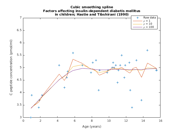
The data, given by
Hastie and Tibshirani (1990), is the age,
, and C-peptide concentration (pmol/ml),
, from a study of the factors affecting insulin-dependent diabetes mellitus in children. The data is input, reduced to a strictly ordered set by
nag_smooth_data_order (g10za) and a series of splines fit using a range of values for the smoothing parameter,
.
Open in the MATLAB editor:
g10ab_example
function g10ab_example
fprintf('g10ab example results\n\n');
x = [ 5.2 8.8 10.5 10.6 10.4 1.8 12.7 15.6 5.8 1.9 ...
2.2 4.8 7.9 5.2 0.9 11.8 7.9 11.5 10.6 8.5 ...
11.1 12.8 11.3 1.0 14.5 11.9 8.1 13.8 15.5 9.8 ...
11.0 12.4 11.1 5.1 4.8 4.2 6.9 13.2 9.9 12.5 ...
13.2 8.9 10.8];
y = [ 4.8 4.1 5.2 5.5 5.0 3.4 3.4 4.9 5.6 3.7 ...
3.9 4.5 4.8 4.9 3.0 4.6 4.8 5.5 4.5 5.3 ...
4.7 6.6 5.1 3.9 5.7 5.1 5.2 3.7 4.9 4.8 ...
4.4 5.2 5.1 4.6 3.9 5.1 5.1 6.0 4.9 4.1 ...
4.6 4.9 5.1];
[n, x, y, wt, rss, ifail] = g10za( ...
x, y);
x = x(1:n);
y = y(1:n);
rho = [1 10 100];
nrho = numel(rho);
c = zeros(n, 3);
comm = zeros(9*n+14, 1);
yhat = zeros(n,nrho);
rss = zeros(nrho,1);
df = zeros(nrho,1);
mode = 'P';
[yhat(:,1), c, rss(1), df(1), res, h, comm, ifail] = ...
g10ab(mode, x, y, rho(1), c, comm, 'wt', wt);
mode = 'Q';
for j = 2:nrho
[yhat(:,j), c, rss(j), df(j), res, h, comm, ifail] = ...
g10ab( ...
mode, x, y, rho(j), c, comm, 'wt', wt);
end
fprintf('Smoothing coefficient (rho) = ');
fprintf(' %8.2f', rho);
fprintf('\nResidual sum of squares = ');
fprintf('%10.3f', rss);
fprintf('\nDegrees of freedom = ');
fprintf('%10.3f', df);
fprintf('\n\n x y Fitted Values\n');
fprintf('%8.4f%8.4f%24.4f%10.4f%10.4f\n', [x y yhat]');
fig1 = figure;
plot(x,y,'+',x,yhat(:,1),x,yhat(:,2),x,yhat(:,3));
legend('Raw data', '\rho = 1', '\rho = 10', '\rho = 100', ...
'Location','NorthWest');
xlabel('Age (years)');
ylabel('C-peptide concentration (pmol/ml)');
title({'Cubic smoothing spline', ...
'Factors affecting insulin-dependent diabetis mellitus', ...
'in children; Hastie and Tibshirani (1990)'});
g10ab example results

Smoothing coefficient (rho) =       1.00     10.00    100.00
Residual sum of squares     =      9.118    11.288    11.881
Degrees of freedom          =     22.505    27.785    31.191

    x       y                            Fitted Values
  0.9000  3.0000                  3.3784    3.3674    3.3699
  1.0000  3.9000                  3.4173    3.4008    3.4063
  1.8000  3.4000                  3.6144    3.6642    3.6973
  1.9000  3.7000                  3.6639    3.7016    3.7341
  2.2000  3.9000                  3.8607    3.8214    3.8449
  4.2000  5.1000                  4.7441    4.5265    4.5194
  4.8000  4.2000                  4.4914    4.6471    4.6746
  5.1000  4.6000                  4.6708    4.7561    4.7470
  5.2000  4.8500                  4.7704    4.7993    4.7702
  5.8000  5.6000                  5.3426    5.0458    4.8879
  6.9000  5.1000                  5.1728    5.1204    4.9753
  7.9000  4.8000                  4.9467    4.9590    4.9537
  8.1000  5.2000                  4.9556    4.9262    4.9452
  8.5000  5.3000                  4.8742    4.8595    4.9276
  8.8000  4.1000                  4.7305    4.8172    4.9168
  8.9000  4.9000                  4.7024    4.8095    4.9143
  9.8000  4.8000                  4.8394    4.8676    4.9170
  9.9000  4.9000                  4.8746    4.8818    4.9191
 10.4000  5.0000                  4.9971    4.9445    4.9303
 10.5000  5.2000                  4.9997    4.9521    4.9321
 10.6000  5.0000                  4.9921    4.9572    4.9335
 10.8000  5.1000                  4.9603    4.9613    4.9354
 11.0000  4.4000                  4.9396    4.9614    4.9363
 11.1000  4.9000                  4.9494    4.9618    4.9366
 11.3000  5.1000                  4.9926    4.9623    4.9366
 11.5000  5.5000                  5.0116    4.9568    4.9355
 11.8000  4.6000                  4.9372    4.9338    4.9315
 11.9000  5.1000                  4.9042    4.9251    4.9300
 12.4000  5.2000                  4.7929    4.8943    4.9240
 12.5000  4.1000                  4.8042    4.8944    4.9237
 12.7000  3.4000                  4.9020    4.9051    4.9244
 12.8000  6.6000                  4.9752    4.9138    4.9252
 13.2000  5.3000                  5.0173    4.9239    4.9276
 13.8000  3.7000                  4.6164    4.8930    4.9304
 14.5000  5.7000                  5.1883    4.9938    4.9518
 15.5000  4.9000                  4.9854    4.9773    4.9687
 15.6000  4.9000                  4.9167    4.9682    4.9697

PDF version (NAG web site
, 64-bit version, 64-bit version)
© The Numerical Algorithms Group Ltd, Oxford, UK. 2009–2015
