nag_fit_2dcheb_lines (e02ca) forms an approximation to the weighted, least squares Chebyshev series surface fit to data arbitrarily distributed on lines parallel to one independent coordinate axis.

Syntax

[a, ifail] = e02ca(m, k, l, x, y, f, w, xmin, xmax, nux, nuy, 'n', n, 'inuxp1', inuxp1, 'inuyp1', inuyp1)

[a, ifail] = nag_fit_2dcheb_lines(m, k, l, x, y, f, w, xmin, xmax, nux, nuy, 'n', n, 'inuxp1', inuxp1, 'inuyp1', inuyp1)

Description

nag_fit_2dcheb_lines (e02ca) determines a bivariate polynomial approximation of degree

k

x

and

l

y

to the set of data points

(x_{r, s}, y_{s}, f_{r, s})

, with weights

w_{r, s}

, for

s = 1, 2, \dots, n

and

r = 1, 2, \dots, m_{s}

. That is, the data points are on lines

y = y_{s}

, but the

x

values may be different on each line. The values of

k

and

l

are prescribed by you (for guidance on their choice, see Further Comments). The function is based on the method described in Sections 5 and 6 of Clenshaw and Hayes (1965).

The polynomial is represented in double Chebyshev series form with arguments

\bar{x}

and

\bar{y}

. The arguments lie in the range

- 1

+ 1

and are related to the original variables

x

and

y

by the transformations

\bar{x} = \frac{2 x - (x_{\max} + x_{\min})}{(x_{\max} - x_{\min})} and \bar{y} = \frac{2 y - (y_{\max} + y_{\min})}{(y_{\max} - y_{\min})} .

Here

y_{\max}

and

y_{\min}

are set by the function to, respectively, the largest and smallest value of

y_{s}

, but

x_{\max}

and

x_{\min}

are functions of

y

prescribed by you (see Further Comments). For this function, only their values

x_{\max}^{(s)}

and

x_{\min}^{(s)}

at each

y = y_{s}

are required. For each

s = 1, 2, \dots, n

x_{\max}^{(s)}

must not be less than the largest

x_{r, s}

on the line

y = y_{s}

, and, similarly,

x_{\min}^{(s)}

must not be greater than the smallest

x_{r, s}

The double Chebyshev series can be written as

\sum_{i = 0}^{k} \sum_{j = 0}^{l} a_{i j} T_{i} (\bar{x}) T_{j} (\bar{y})

where

T_{i} (\bar{x})

is the Chebyshev polynomial of the first kind of degree

i

with argument

\bar{x}

, and

T_{j} (y)

is similarly defined. However, the standard convention, followed in this function, is that coefficients in the above expression which have either

i

j

zero are written as

\frac{1}{2} a_{i j}

, instead of simply

a_{i j}

, and the coefficient with both

i

and

j

equal to zero is written as

\frac{1}{4} a_{0, 0}

. The series with coefficients output by the function should be summed using this convention. nag_fit_2dcheb_eval (e02cb) is available to compute values of the fitted function from these coefficients.

The function first obtains Chebyshev series coefficients

c_{s, i}

, for

i = 0, 1, \dots, k

, of the weighted least squares polynomial curve fit of degree

k

\bar{x}

to the data on each line

y = y_{s}

, for

s = 1, 2, \dots, n

, in turn, using an auxiliary function. The same function is then called

k + 1

times to fit

c_{s, i}

, for

s = 1, 2, \dots, n

, by a polynomial of degree

l

\bar{y}

, for each

i = 0, 1, \dots, k

. The resulting coefficients are the required

a_{i j}

You can force the fit to contain a given polynomial factor. This allows for the surface fit to be constrained to have specified values and derivatives along the boundaries

x = x_{\min}

x = x_{\max}

y = y_{\min}

and

y = y_{\max}

or indeed along any lines

\bar{x} =

constant or

\bar{y} =

constant (see Section 8 of Clenshaw and Hayes (1965)).

References

Clenshaw C W and Hayes J G (1965) Curve and surface fitting J. Inst. Math. Appl. 1 164–183

Hayes J G (ed.) (1970) Numerical Approximation to Functions and Data Athlone Press, London

Parameters

Compulsory Input Parameters

1: $m (n)$ – int64int32nag_int array

m (s)

must be set to

m_{s}

, the number of data

x

values on the line

y = y_{s}

, for

s = 1, 2, \dots, n

Constraint:

m (s) > 0

, for

s = 1, 2, \dots, n

2: $k$ – int64int32nag_int scalar

k

, the required degree of

x

in the fit.

Constraint: for

s = 1, 2, \dots, n

inuxp1 - 1 \leq k < mdist (s) + inuxp1 - 1

, where

mdist (s)

is the number of distinct

x

values with nonzero weight on the line

y = y_{s}

. See Further Comments.

3: $l$ – int64int32nag_int scalar

l

, the required degree of

y

in the fit.

Constraints:

$l \geq 0$ ;
$inuyp1 - 1 \leq l < n + inuyp1 - 1$ .

4: $x (mtot)$ – double array

mtot, the dimension of the array, must satisfy the constraint

mtot \geq \sum_{s = 1}^{n} m (s)

The

x

values of the data points. The sequence must be

all points on $y = y_{1}$ , followed by
all points on $y = y_{2}$ , followed by
$⋮$
all points on $y = y_{n}$ .

Constraint: for each

y_{s}

, the

x

values must be in nondecreasing order.

5: $y (n)$ – double array

y (s)

must contain the

y

value of line

y = y_{s}

, for

s = 1, 2, \dots, n

, on which data is given.

Constraint: the

y_{s}

values must be in strictly increasing order.

6: $f (mtot)$ – double array

mtot, the dimension of the array, must satisfy the constraint

mtot \geq \sum_{s = 1}^{n} m (s)

f

, the data values of the dependent variable in the same sequence as the

x

values.

7: $w (mtot)$ – double array

mtot, the dimension of the array, must satisfy the constraint

mtot \geq \sum_{s = 1}^{n} m (s)

The weights to be assigned to the data points, in the same sequence as the

x

values. These weights should be calculated from estimates of the absolute accuracies of the

f_{r}

, expressed as standard deviations, probable errors or some other measure which is of the same dimensions as

f_{r}

. Specifically, each

w_{r}

should be inversely proportional to the accuracy estimate of

f_{r}

. Often weights all equal to unity will be satisfactory. If a particular weight is zero, the corresponding data point is omitted from the fit.

8: $xmin (n)$ – double array

xmin (s)

must contain

x_{\min}^{(s)}

, the lower end of the range of

x

on the line

y = y_{s}

, for

s = 1, 2, \dots, n

. It must not be greater than the lowest data value of

x

on the line. Each

x_{\min}^{(s)}

is scaled to

- 1.0

in the fit. (See also Further Comments.)

9: $xmax (n)$ – double array

xmax (s)

must contain

x_{\max}^{(s)}

, the upper end of the range of

x

on the line

y = y_{s}

, for

s = 1, 2, \dots, n

. It must not be less than the highest data value of

x

on the line. Each

x_{\max}^{(s)}

is scaled to

+ 1.0

in the fit. (See also Further Comments.)

Constraint:

xmax (s) > xmin (s)

10: $nux (inuxp1)$ – double array

nux (i)

must contain the coefficient of the Chebyshev polynomial of degree

(i - 1)

\bar{x}

, in the Chebyshev series representation of the polynomial factor in

\bar{x}

which you require the fit to contain, for

i = 1, 2, \dots, inuxp1

. These coefficients are defined according to the standard convention of Description.

Constraint:

nux (inuxp1)

must be nonzero, unless

inuxp1 = 1

, in which case nux is ignored.

11: $nuy (inuyp1)$ – double array

nuy (i)

must contain the coefficient of the Chebyshev polynomial of degree

(i - 1)

\bar{y}

, in the Chebyshev series representation of the polynomial factor which you require the fit to contain, for

i = 1, 2, \dots, inuyp1

. These coefficients are defined according to the standard convention of Description.

Constraint:

nuy (inuyp1)

must be nonzero, unless

inuyp1 = 1

, in which case nuy is ignored.

Optional Input Parameters

1: $n$ – int64int32nag_int scalar: Default: the dimension of the arrays m, y, xmin, xmax. (An error is raised if these dimensions are not equal.)
The number of lines $y =$ constant on which data points are given.

Constraint: $n > 0$ .
2: $inuxp1$ – int64int32nag_int scalar: Default: the dimension of the array nux.
$inux + 1$ , where $inux$ is the degree of a polynomial factor in $\bar{x}$ which you require the fit to contain. (See Description, last paragraph.)
If this option is not required, inuxp1 should be set equal to $1$ .

Constraint: $1 \leq inuxp1 \leq k + 1$ .
3: $inuyp1$ – int64int32nag_int scalar: Default: the dimension of the array nuy.
$inuy + 1$ , where $inuy$ is the degree of a polynomial factor in $\bar{y}$ which you require the fit to contain. (See Description, last paragraph.) If this option is not required, inuyp1 should be set equal to $1$ .

Output Parameters

1: $a (na)$ – double array: $na = (k + 1) \times (l + 1)$ , the total number of coefficients in the fit.
Contains the Chebyshev coefficients of the fit. $a (i \times (l + 1) + j)$ is the coefficient $a_{i j}$ of Description defined according to the standard convention. These coefficients are used by nag_fit_2dcheb_eval (e02cb) to calculate values of the fitted function.
2: $ifail$ – int64int32nag_int scalar: $ifail = 0$ unless the function detects an error (see Error Indicators and Warnings).

Error Indicators and Warnings

Errors or warnings detected by the function:

$ifail = 1$

On entry,	k or $l < 0$ ,
or	inuxp1 or $inuyp1 < 1$ ,
or	$inuxp1 > k + 1$ ,
or	$inuyp1 > l + 1$ ,
or	$m (i) < k - inuxp1 + 2$ for some $i = 1, 2, \dots, n$ ,
or	$n < l - inuyp1 + 2$ ,
or	na is too small,
or	nwork is too small,
or	mtot is too small.

$ifail = 2$: $xmin (i)$ and $xmax (i)$ do not span the data x values on $y = y (i)$ for some $i = 1, 2, \dots, n$ , possibly because $xmin (i) \geq xmax (i)$ .

$ifail = 3$: The data x values on $y = y (i)$ are not nondecreasing for some $i = 1, 2, \dots, n$ , or the $y (i)$ themselves are not strictly increasing.

$ifail = 4$: The number of distinct x values with nonzero weight on $y = y (i)$ is less than $k - inuxp1 + 2$ for some $i = 1, 2, \dots, n$ .

$ifail = 5$

On entry,	$nux (inuxp1) = 0.0$ and $inuxp1 \neq 1$ ,
or	$nuy (inuyp1) = 0.0$ and $inuyp1 \neq 1$ .

$ifail = - 99$: An unexpected error has been triggered by this routine. Please contact NAG.

$ifail = - 399$: Your licence key may have expired or may not have been installed correctly.

$ifail = - 999$: Dynamic memory allocation failed.

Accuracy

No error analysis for this method has been published. Practical experience with the method, however, is generally extremely satisfactory.

Further Comments

The time taken is approximately proportional to

k \times (k \times mtot + n \times l^{2})

The reason for allowing

x_{\max}

and

x_{\min}

(which are used to normalize the range of

x

) to vary with

y

is that unsatisfactory fits can result if the highest (or lowest) data values of the normalized

x

on each line

y = y_{s}

are not approximately the same. (For an explanation of this phenomenon, see page 176 of Clenshaw and Hayes (1965).) Commonly in practice, the lowest (for example) data values

x_{1, s}

, while not being approximately constant, do lie close to some smooth curve in the

(x, y)

plane. Using values from this curve as the values of

x_{\min}

, different in general on each line, causes the lowest transformed data values

{\bar{x}}_{1, s}

to be approximately constant. Sometimes, appropriate curves for

x_{\max}

and

x_{\min}

will be clear from the context of the problem (they need not be polynomials). If this is not the case, suitable curves can often be obtained by fitting to the lowest data values

x_{1, s}

and to the corresponding highest data values of

x

, low degree polynomials in

y

, using function nag_fit_1dcheb_arb (e02ad), and then shifting the two curves outwards by a small amount so that they just contain all the data between them. The complete curves are not in fact supplied to the present function, only their values at each

y_{s}

; and the values simply need to lie on smooth curves. More values on the complete curves will be required subsequently, when computing values of the fitted surface at arbitrary

y

values.

Naturally, a satisfactory approximation to the surface underlying the data cannot be expected if the character of the surface is not adequately represented by the data. Also, as always with polynomials, the approximating function may exhibit unwanted oscillations (particularly near the ends of the ranges) if the degrees

k

and

l

are taken greater than certain values, generally unknown but depending on the total number of coefficients

(k + 1) \times (l + 1)

should be significantly smaller than, say not more than half, the total number of data points. Similarly,

k + 1

should be significantly smaller than most (preferably all) the

m_{s}

, and

l + 1

significantly smaller than

n

. Closer spacing of the data near the ends of the

x

and

y

ranges is an advantage. In particular, if

{\bar{y}}_{s} = - \cos (π (s - 1) / (n - 1))

, for

s = 1, 2, \dots, n

and

{\bar{x}}_{r, s} = - \cos (π (r - 1) / (m - 1))

, for

r = 1, 2, \dots, m

, (thus

m_{s} = m

for all

s

), then the values

k = m - 1

and

l = n - 1

(so that the polynomial passes exactly through all the data points) should not give unwanted oscillations. Other datasets should be similarly satisfactory if they are everywhere at least as closely spaced as the above cosine values with

m

replaced by

k + 1

and

n

l + 1

(more precisely, if for every

s

the largest interval between consecutive values of

\arccos {\bar{x}}_{r, s}

, for

r = 1, 2, \dots, m

, is not greater than

π / k

, and similarly for the

{\bar{y}}_{s}

). The polynomial obtained should always be examined graphically before acceptance. Note that, for this purpose it is not sufficient to plot the polynomial only at the data values of

x

and

y

: intermediate values should also be plotted, preferably via a graphics facility.

Provided the data are adequate, and the surface underlying the data is of a form that can be represented by a polynomial of the chosen degrees, the function should produce a good approximation to this surface. It is not, however, the true least squares surface fit nor even a polynomial in

x

and

y

, the original variables (see Section 6 of Clenshaw and Hayes (1965), ), except in certain special cases. The most important of these is where the data values of

x

are the same on each line

y = y_{s}

, (i.e., the data points lie on a rectangular mesh in the

(x, y)

plane), the weights of the data points are all equal, and

x_{\max}

and

x_{\min}

are both constants (in this case they should be set to the largest and smallest data values of

x

, respectively).

If the dataset is such that it can be satisfactorily approximated by a polynomial of degrees

k^{'}

and

l^{'}

, say, then if higher values are used for

k

and

l

in the function, all the coefficients

a_{i j}

for

i > k^{'}

j > l^{'}

will take apparently random values within a range bounded by the size of the data errors, or rather less. (This behaviour of the Chebyshev coefficients, most readily observed if they are set out in a rectangular array, closely parallels that in curve-fitting, examples of which are given in Section 8 of Hayes (1970).) In practice, therefore, to establish suitable values of

k^{'}

and

l^{'}

, you should first be seeking (within the limitations discussed above) values for

k

and

l

which are large enough to exhibit the behaviour described. Values for

k^{'}

and

l^{'}

should then be chosen as the smallest which do not exclude any coefficients significantly larger than the random ones. A polynomial of degrees

k^{'}

and

l^{'}

should then be fitted to the data.

If the option to force the fit to contain a given polynomial factor in

x

is used and if zeros of the chosen factor coincide with data

x

values on any line, then the effective number of data points on that line is reduced by the number of such coincidences. A similar consideration applies when forcing the

y

-direction. No account is taken of this by the function when testing that the degrees

k

and

l

have not been chosen too large.

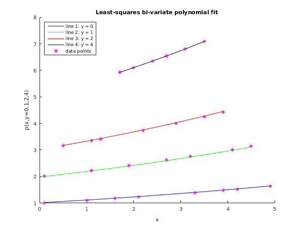
Example

This example reads data in the following order, using the notation of the argument list for nag_fit_2dcheb_lines (e02ca) above:

\begin{array}{l} n k l \\ y (i) m (i) xmin (i) xmax (i), & for ​ i = 1, 2, \dots, n \\ x (i) f (i) w (i), & for ​ i = 1, 2, \dots, mtot . \end{array}

The data points are fitted using nag_fit_2dcheb_lines (e02ca), and then the fitting polynomial is evaluated at the data points using nag_fit_2dcheb_eval (e02cb).

The output is:

the data points and their fitted values;
the Chebyshev coefficients of the fit.

Open in the MATLAB editor: e02ca_example

function e02ca_example


fprintf('e02ca example results\n\n');

% Fit cubic in x and quadratic in y
k = int64(3);
l = int64(2);

% 4 lines of data, 1 for each of 4 values of y
n = 4;
m = int64([8 7 7 6]);
mtot = sum(m);
x = [0.1     1.0     1.6     2.1     3.3     3.9     4.2     4.9 ...
     0.1     1.1     1.9     2.7     3.2     4.1     4.5         ...
     0.5     1.1     1.3     2.2     2.9     3.5     3.9         ...
     1.7     2.0     2.4     2.7     3.1     3.5 ];
f = [1.01005 1.10517 1.17351 1.23368 1.39097 1.47698 1.52196 1.63232 ...
     2.02010 2.23256 2.41850 2.61993 2.75426 3.01364 3.13662         ...
     3.15381 3.34883 3.41649 3.73823 4.00928 4.25720 4.43094         ...
     5.92652 6.10701 6.35625 6.54982 6.81713 7.09534 ];
w =  ones(mtot, 1);

y    = [0   1    2    4  ];  ymin = min(y); ymax = max(y);
xmin = [0   0.1  0.4  1.6];
xmax = [5   4.5  4    3.5];

nux  = [0];
nuy  = nux;

% Compute surface fit
[a, ifail] = e02ca( ...
                    m, k, l, x, y, f, w, xmin, xmax, nux, nuy);

fig1 = figure;
colors = {'Blue','Green','Red','Black'};
hold on;
% Evaluate fit 
mlast = int64(0);
for i = 1:n
  mfirst = mlast + 1;
  mlast  = mlast + m(i);
  [fit, ifail] = e02cb( ...
                        mfirst, k, l, x, xmin(i), xmax(i), y(i), ...
                        ymin, ymax, a, 'mlast', mlast);
  mm = mfirst:mlast;
  mfit(mm) = fit(mm);

  fprintf('\nLine number %d, y = %7.2f\n',i,y(i));
  fprintf('       x          f         fit      residual\n');
  sol = [x(mm); f(mm); fit(mm)'; fit(mm)'-f(mm)];
  fprintf('%11.4f%11.4f%11.4f%11.2e\n', sol);
  col = colors(:,i);
  plot(x(mm),fit(mm),'Color',char(col));
end
plot(x,f,'*','Color','Magenta');
hold off
title('Least-squares bi-variate polynomial fit');
xlabel('x');
ylabel('p(x,y=0,1,2,4)')
legend('line 1: y = 0','line 2: y = 1','line 3: y = 2',...
       'line 4: y = 4','data points','Location','NorthWest');

e02ca example results


Line number 1, y =    0.00
       x          f         fit      residual
     0.1000     1.0100     1.0175   7.40e-03
     1.0000     1.1052     1.1126   7.39e-03
     1.6000     1.1735     1.1809   7.43e-03
     2.1000     1.2337     1.2412   7.55e-03
     3.3000     1.3910     1.3992   8.19e-03
     3.9000     1.4770     1.4857   8.72e-03
     4.2000     1.5220     1.5310   9.03e-03
     4.9000     1.6323     1.6422   9.83e-03

Line number 2, y =    1.00
       x          f         fit      residual
     0.1000     2.0201     1.9987  -2.14e-02
     1.1000     2.2326     2.2110  -2.16e-02
     1.9000     2.4185     2.3962  -2.23e-02
     2.7000     2.6199     2.5966  -2.34e-02
     3.2000     2.7543     2.7299  -2.43e-02
     4.1000     3.0136     2.9869  -2.68e-02
     4.5000     3.1366     3.1084  -2.82e-02

Line number 3, y =    2.00
       x          f         fit      residual
     0.5000     3.1538     3.1700   1.62e-02
     1.1000     3.3488     3.3648   1.60e-02
     1.3000     3.4165     3.4325   1.60e-02
     2.2000     3.7382     3.7549   1.66e-02
     2.9000     4.0093     4.0272   1.79e-02
     3.5000     4.2572     4.2769   1.97e-02
     3.9000     4.4309     4.4521   2.12e-02

Line number 4, y =    4.00
       x          f         fit      residual
     1.7000     5.9265     5.9231  -3.42e-03
     2.0000     6.1070     6.1036  -3.41e-03
     2.4000     6.3563     6.3527  -3.50e-03
     2.7000     6.5498     6.5462  -3.64e-03
     3.1000     6.8171     6.8132  -3.98e-03
     3.5000     7.0953     7.0909  -4.49e-03

PDF version (NAG web site, 64-bit version, 64-bit version)

Chapter Contents

Chapter Introduction

NAG Toolbox