PDF version (NAG web site
, 64-bit version, 64-bit version)
NAG Toolbox: nag_fit_2dcheb_eval (e02cb)
Purpose
nag_fit_2dcheb_eval (e02cb) evaluates a bivariate polynomial from the rectangular array of coefficients in its double Chebyshev series representation.
Syntax
[
ff,
ifail] = e02cb(
mfirst,
k,
l,
x,
xmin,
xmax,
y,
ymin,
ymax,
a, 'mlast',
mlast)
[
ff,
ifail] = nag_fit_2dcheb_eval(
mfirst,
k,
l,
x,
xmin,
xmax,
y,
ymin,
ymax,
a, 'mlast',
mlast)
Description
This function evaluates a bivariate polynomial (represented in double Chebyshev form) of degree
in one variable,
, and degree
in the other,
. The range of both variables is
to
. However, these normalized variables will usually have been derived (as when the polynomial has been computed by
nag_fit_2dcheb_lines (e02ca), for example) from your original variables
and
by the transformations
(Here
and
are the ends of the range of
which has been transformed to the range
to
of
.
and
are correspondingly for
. See
Further Comments). For this reason, the function has been designed to accept values of
and
rather than
and
, and so requires values of
, etc. to be supplied by you. In fact, for the sake of efficiency in appropriate cases, the function evaluates the polynomial for a sequence of values of
, all associated with the same value of
.
The double Chebyshev series can be written as
where
is the Chebyshev polynomial of the first kind of degree
and argument
, and
is similarly defined. However the standard convention, followed in this function, is that coefficients in the above expression which have either
or
zero are written
, instead of simply
, and the coefficient with both
and
zero is written
.
The function first forms
, with
replaced by
, for each of
. The value of the double series is then obtained for each value of
, by summing
, with
replaced by
, over
. The Clenshaw three term recurrence (see
Clenshaw (1955)) with modifications due to Reinsch and
Gentleman (1969) is used to form the sums.
References
Clenshaw C W (1955) A note on the summation of Chebyshev series Math. Tables Aids Comput. 9 118–120
Gentleman W M (1969) An error analysis of Goertzel's (Watt's) method for computing Fourier coefficients Comput. J. 12 160–165
Parameters
Compulsory Input Parameters
- 1:
– int64int32nag_int scalar
-
The index of the first and last
value in the array
at which the evaluation is required respectively (see
Further Comments).
Constraint:
.
- 2:
– int64int32nag_int scalar
- 3:
– int64int32nag_int scalar
-
The degree of and of , respectively, in the polynomial.
Constraint:
and .
- 4:
– double array
-
, for , must contain the values at which the evaluation is required.
Constraint:
, for all .
- 5:
– double scalar
- 6:
– double scalar
-
The lower and upper ends,
and
, of the range of the variable
(see
Description).
The values of
xmin and
xmax may depend on the value of
(e.g., when the polynomial has been derived using
nag_fit_2dcheb_lines (e02ca)).
Constraint:
.
- 7:
– double scalar
-
The value of the coordinate of all the points at which the evaluation is required.
Constraint:
.
- 8:
– double scalar
- 9:
– double scalar
-
The lower and upper ends,
and
, of the range of the variable
(see
Description).
Constraint:
.
- 10:
– double array
-
na, the dimension of the array, must satisfy the constraint
, the number of coefficients in a polynomial of the specified degree.
The Chebyshev coefficients of the polynomial. The coefficient
defined according to the standard convention (see
Description) must be in
.
Optional Input Parameters
- 1:
– int64int32nag_int scalar
-
Default:
For
mlast, the dimension of the array
x.
The index of the first and last
value in the array
at which the evaluation is required respectively (see
Further Comments).
Constraint:
.
Output Parameters
- 1:
– double array
-
gives the value of the polynomial at the point , for .
- 2:
– int64int32nag_int scalar
unless the function detects an error (see
Error Indicators and Warnings).
Error Indicators and Warnings
Errors or warnings detected by the function:
-
-
| On entry, | , |
| or | , |
| or | , |
| or | , |
| or | . |
-
-
| On entry, | , |
| or | , |
| or | . |
-
-
| On entry, | , |
| or | , or , for some . |
-
An unexpected error has been triggered by this routine. Please
contact
NAG.
-
Your licence key may have expired or may not have been installed correctly.
-
Dynamic memory allocation failed.
Accuracy
The method is numerically stable in the sense that the computed values of the polynomial are exact for a set of coefficients which differ from those supplied by only a modest multiple of
machine precision.
Further Comments
The time taken is approximately proportional to , where , the number of points at which the evaluation is required.
This function is suitable for evaluating the polynomial surface fits produced by the function
nag_fit_2dcheb_lines (e02ca), which provides the
double
array
a in the required form. For this use, the values of
and
supplied to the present function must be the same as those supplied to
nag_fit_2dcheb_lines (e02ca). The same applies to
and
if they are independent of
. If they vary with
, their values must be consistent with those supplied to
nag_fit_2dcheb_lines (e02ca) (see
Further Comments in
nag_fit_2dcheb_lines (e02ca)).
The arguments
mfirst and
mlast are intended to permit the selection of a segment of the array
x which is to be associated with a particular value of
, when, for example, other segments of
x are associated with other values of
. Such a case arises when, after using
nag_fit_2dcheb_lines (e02ca) to fit a set of data, you wish to evaluate the resulting polynomial at all the data values. In this case, if the arguments
x,
y,
mfirst and
mlast of the present function are set respectively (in terms of arguments of
nag_fit_2dcheb_lines (e02ca)) to
x,
,
and
, the function will compute values of the polynomial surface at all data points which have
as their
coordinate (from which values the residuals of the fit may be derived).
Example
This example reads data in the following order, using the notation of the argument list above:
For each line
the polynomial is evaluated at
equispaced points between
and
inclusive.
Open in the MATLAB editor:
e02cb_example
function e02cb_example
fprintf('e02cb example results\n\n');
dx = 4/19;
x = [0.5:dx:4.5];
y = [0:dx:4];
xmin = 0.1; xmax = 4.5;
ymin = 0; ymax = 4;
k = int64(3);
l = int64(2);
a = [15.3482 5.15073 -2.20140 1.14719 -0.64419 0.30464 ...
-0.4901 -0.00314 -6.69912 0.00153 3.00033 -0.00022];
mfirst = int64(1);
mlast = int64(20);
for i = 1:mlast
[fit(:,i), ifail] = e02cb( ...
mfirst, k, l, x, xmin, xmax, y(i), ...
ymin, ymax, a, 'mlast', mlast);
sol = [x; fit(:,i)'];
end
fprintf('\nThe bivariate polynomial fit values for y = %5.1f are:\n',y(mlast));
sol = [x; fit(:,mlast)'];
fprintf(' x p(x,y=4)\n', sol);
fprintf('%11.4f%11.4f\n', sol);
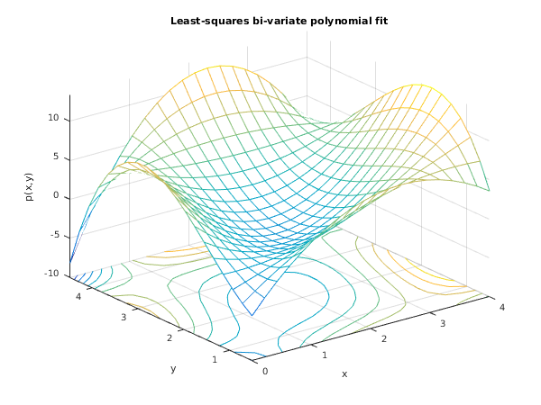
fig1 = figure;
meshc(y,x,fit);
title('Least-squares bi-variate polynomial fit');
xlabel('x');
ylabel('y');
zlabel('p(x,y)');
e02cb example results


The bivariate polynomial fit values for y =   4.0 are:
      x       p(x,y=4)
     0.5000     3.5575
     0.7105     6.8145
     0.9211     9.3405
     1.1316    11.1986
     1.3421    12.4520
     1.5526    13.1637
     1.7632    13.3970
     1.9737    13.2148
     2.1842    12.6803
     2.3947    11.8566
     2.6053    10.8069
     2.8158     9.5942
     3.0263     8.2816
     3.2368     6.9323
     3.4474     5.6094
     3.6579     4.3760
     3.8684     3.2951
     4.0789     2.4300
     4.2895     1.8437
     4.5000     1.5993
PDF version (NAG web site
, 64-bit version, 64-bit version)
© The Numerical Algorithms Group Ltd, Oxford, UK. 2009–2015
