nag_pde_1d_parab_convdiff_dae (d03pl) integrates a system of linear or nonlinear convection-diffusion equations in one space dimension, with optional source terms and scope for coupled ordinary differential equations (ODEs). The system must be posed in conservative form. Convection terms are discretized using a sophisticated upwind scheme involving a user-supplied numerical flux function based on the solution of a Riemann problem at each mesh point. The method of lines is employed to reduce the partial differential equations (PDEs) to a system of ODEs, and the resulting system is solved using a backward differentiation formula (BDF) method or a Theta method.

Syntax

[ts, u, rsave, isave, ind, ifail] = d03pl(npde, ts, tout, pdedef, numflx, bndary, u, x, ncode, odedef, xi, rtol, atol, itol, norm_p, laopt, algopt, rsave, isave, itask, itrace, ind, 'npts', npts, 'nxi', nxi, 'neqn', neqn)

[ts, u, rsave, isave, ind, ifail] = nag_pde_1d_parab_convdiff_dae(npde, ts, tout, pdedef, numflx, bndary, u, x, ncode, odedef, xi, rtol, atol, itol, norm_p, laopt, algopt, rsave, isave, itask, itrace, ind, 'npts', npts, 'nxi', nxi, 'neqn', neqn)

Note: the interface to this routine has changed since earlier releases of the toolbox:

At Mark 22:

lrsave and lisave were removed from the interface

Description

nag_pde_1d_parab_convdiff_dae (d03pl) integrates the system of convection-diffusion equations in conservative form:

\sum_{j = 1}^{npde} P_{i, j} \frac{\partial U_{j}}{\partial t} + \frac{\partial F_{i}}{\partial x} = C_{i} \frac{\partial D_{i}}{\partial x} + S_{i},

(1)

or the hyperbolic convection-only system:

\frac{\partial U_{i}}{\partial t} + \frac{\partial F_{i}}{\partial x} = 0,

(2)

for

i = 1, 2, \dots, npde, a \leq x \leq b, t \geq t_{0}

, where the vector

U

is the set of PDE solution values

U (x, t) = {[U_{1} (x, t), \dots, U_{npde} (x, t)]}^{T} .

The optional coupled ODEs are of the general form

R_{i} (t, V, \dot{V}, ξ, U^{*}, U_{x}^{*}, U_{t}^{*}) = 0, i = 1, 2, \dots, ncode,

(3)

where the vector

V

is the set of ODE solution values

V (t) = {[V_{1} (t), \dots, V_{ncode} (t)]}^{T},

\dot{V}

denotes its derivative with respect to time, and

U_{x}

is the spatial derivative of

U

In (1),

P_{i, j}

F_{i}

and

C_{i}

depend on

x

t

U

and

V

;

D_{i}

depends on

x

t

U

U_{x}

and

V

; and

S_{i}

depends on

x

t

U

V

and linearly on

\dot{V}

. Note that

P_{i, j}

F_{i}

C_{i}

and

S_{i}

must not depend on any space derivatives, and

P_{i, j}

F_{i}

C_{i}

and

D_{i}

must not depend on any time derivatives. In terms of conservation laws,

F_{i}

\frac{C_{i} \partial D_{i}}{\partial x}

and

S_{i}

are the convective flux, diffusion and source terms respectively.

In (3),

ξ

represents a vector of

n_{ξ}

spatial coupling points at which the ODEs are coupled to the PDEs. These points may or may not be equal to PDE spatial mesh points.

U^{*}

U_{x}^{*}

and

U_{t}^{*}

are the functions

U

U_{x}

and

U_{t}

evaluated at these coupling points. Each

R_{i}

may depend only linearly on time derivatives. Hence (3) may be written more precisely as

R = L - M \dot{V} - N U_{t}^{*},

(4)

where

R = {[R_{1}, \dots, R_{ncode}]}^{T}

L

is a vector of length ncode,

M

is an ncode by ncode matrix,

N

is an ncode by

(n_{ξ} \times npde)

matrix and the entries in

L

M

and

N

may depend on

t

ξ

U^{*}

U_{x}^{*}

and

V

. In practice you only need to supply a vector of information to define the ODEs and not the matrices

L

M

and

N

. (See Arguments for the specification of odedef.)

The integration in time is from

t_{0}

t_{out}

, over the space interval

a \leq x \leq b

, where

a = x_{1}

and

b = x_{npts}

are the leftmost and rightmost points of a user-defined mesh

x_{1}, x_{2}, \dots, x_{npts}

. The initial values of the functions

U (x, t)

and

V (t)

must be given at

t = t_{0}

The PDEs are approximated by a system of ODEs in time for the values of

U_{i}

at mesh points using a spatial discretization method similar to the central-difference scheme used in nag_pde_1d_parab_fd (d03pc), nag_pde_1d_parab_dae_fd (d03ph) and nag_pde_1d_parab_remesh_fd (d03pp), but with the flux

F_{i}

replaced by a numerical flux, which is a representation of the flux taking into account the direction of the flow of information at that point (i.e., the direction of the characteristics). Simple central differencing of the numerical flux then becomes a sophisticated upwind scheme in which the correct direction of upwinding is automatically achieved.

The numerical flux vector,

{\hat{F}}_{i}

say, must be calculated by you in terms of the left and right values of the solution vector

U

(denoted by

U_{L}

and

U_{R}

respectively), at each mid-point of the mesh

x_{j - \frac{1}{2}} = (x_{j - 1} + x_{j}) / 2

, for

j = 2, 3, \dots, npts

. The left and right values are calculated by nag_pde_1d_parab_convdiff_dae (d03pl) from two adjacent mesh points using a standard upwind technique combined with a Van Leer slope-limiter (see LeVeque (1990)). The physically correct value for

{\hat{F}}_{i}

is derived from the solution of the Riemann problem given by

\frac{\partial U_{i}}{\partial t} + \frac{\partial F_{i}}{\partial y} = 0,

(5)

where

y = x - x_{j - \frac{1}{2}}

, i.e.,

y = 0

corresponds to

x = x_{j - \frac{1}{2}}

, with discontinuous initial values

U = U_{L}

for

y < 0

and

U = U_{R}

for

y > 0

, using an approximate Riemann solver. This applies for either of the systems (1) or (2); the numerical flux is independent of the functions

P_{i, j}

C_{i}

D_{i}

and

S_{i}

. A description of several approximate Riemann solvers can be found in LeVeque (1990) and Berzins et al. (1989). Roe's scheme (see Roe (1981)) is perhaps the easiest to understand and use, and a brief summary follows. Consider the system of PDEs

U_{t} + F_{x} = 0

or equivalently

U_{t} + A U_{x} = 0

. Provided the system is linear in

U

, i.e., the Jacobian matrix

A

does not depend on

U

, the numerical flux

\hat{F}

is given by

\hat{F} = \frac{1}{2} (F_{L} + F_{R}) - \frac{1}{2} \sum_{k = 1}^{npde} α_{k} |λ_{k}| e_{k},

(6)

where

F_{L}

(

F_{R}

) is the flux

F

calculated at the left (right) value of

U

, denoted by

U_{L}

(

U_{R}

); the

λ_{k}

are the eigenvalues of

A

; the

e_{k}

are the right eigenvectors of

A

; and the

α_{k}

are defined by

U_{R} - U_{L} = \sum_{k = 1}^{npde} α_{k} e_{k} .

(7)

An example is given in Example and in the nag_pde_1d_parab_convdiff (d03pf) documentation.

If the system is nonlinear, Roe's scheme requires that a linearized Jacobian is found (see Roe (1981)).

The functions

P_{i, j}

C_{i}

D_{i}

and

S_{i}

(but not

F_{i}

) must be specified in pdedef. The numerical flux

{\hat{F}}_{i}

must be supplied in a separate numflx. For problems in the form (2), the actual argument nag_pde_1d_parab_convdiff_dae_sample_pdedef (d03plp) may be used for pdedef. nag_pde_1d_parab_convdiff_dae_sample_pdedef (d03plp) is included in the NAG Toolbox and sets the matrix with entries

P_{i, j}

to the identity matrix, and the functions

C_{i}

D_{i}

and

S_{i}

to zero.

The boundary condition specification has sufficient flexibility to allow for different types of problems. For second-order problems, i.e.,

D_{i}

depending on

U_{x}

, a boundary condition is required for each PDE at both boundaries for the problem to be well-posed. If there are no second-order terms present, then the continuous PDE problem generally requires exactly one boundary condition for each PDE, that is npde boundary conditions in total. However, in common with most discretization schemes for first-order problems, a numerical boundary condition is required at the other boundary for each PDE. In order to be consistent with the characteristic directions of the PDE system, the numerical boundary conditions must be derived from the solution inside the domain in some manner (see below). You must supply both types of boundary condition, i.e., a total of npde conditions at each boundary point.

The position of each boundary condition should be chosen with care. In simple terms, if information is flowing into the domain then a physical boundary condition is required at that boundary, and a numerical boundary condition is required at the other boundary. In many cases the boundary conditions are simple, e.g., for the linear advection equation. In general you should calculate the characteristics of the PDE system and specify a physical boundary condition for each of the characteristic variables associated with incoming characteristics, and a numerical boundary condition for each outgoing characteristic.

A common way of providing numerical boundary conditions is to extrapolate the characteristic variables from the inside of the domain (note that when using banded matrix algebra the fixed bandwidth means that only linear extrapolation is allowed, i.e., using information at just two interior points adjacent to the boundary). For problems in which the solution is known to be uniform (in space) towards a boundary during the period of integration then extrapolation is unnecessary; the numerical boundary condition can be supplied as the known solution at the boundary. Another method of supplying numerical boundary conditions involves the solution of the characteristic equations associated with the outgoing characteristics. Examples of both methods can be found in Example and in the nag_pde_1d_parab_convdiff (d03pf) documentation.

The boundary conditions must be specified in bndary in the form

G_{i}^{L} (x, t, U, V, \dot{V}) = 0 at ​ x = a, i = 1, 2, \dots, npde,

(8)

at the left-hand boundary, and

G_{i}^{R} (x, t, U, V, \dot{V}) = 0 at ​ x = b, i = 1, 2, \dots, npde,

(9)

at the right-hand boundary.

Note that spatial derivatives at the boundary are not passed explicitly to bndary, but they can be calculated using values of

U

at and adjacent to the boundaries if required. However, it should be noted that instabilities may occur if such one-sided differencing opposes the characteristic direction at the boundary.

The algebraic-differential equation system which is defined by the functions

R_{i}

must be specified in odedef. You must also specify the coupling points

ξ

(if any) in the array xi.

The problem is subject to the following restrictions:

(i)	In (1), ${\dot{V}}_{j} (t)$ , for $j = 1, 2, \dots, ncode$ , may only appear linearly in the functions $S_{i}$ , for $i = 1, 2, \dots, npde$ , with a similar restriction for $G_{i}^{L}$ and $G_{i}^{R}$ ;
(ii)	$P_{i, j}$ , $F_{i}$ , $C_{i}$ and $S_{i}$ must not depend on any space derivatives; and $P_{i, j}$ , $F_{i}$ , $C_{i}$ and $D_{i}$ must not depend on any time derivatives;
(iii)	$t_{0} < t_{out}$ , so that integration is in the forward direction;
(iv)	The evaluation of the terms $P_{i, j}$ , $C_{i}$ , $D_{i}$ and $S_{i}$ is done by calling the pdedef at a point approximately midway between each pair of mesh points in turn. Any discontinuities in these functions must therefore be at one or more of the mesh points $x_{1}, x_{2}, \dots, x_{npts}$ ;
(v)	At least one of the functions $P_{i, j}$ must be nonzero so that there is a time derivative present in the PDE problem.

In total there are

npde \times npts + ncode

ODEs in the time direction. This system is then integrated forwards in time using a BDF or Theta method, optionally switching between Newton's method and functional iteration (see Berzins et al. (1989)).

For further details of the scheme, see Pennington and Berzins (1994) and the references therein.

References

Berzins M, Dew P M and Furzeland R M (1989) Developing software for time-dependent problems using the method of lines and differential-algebraic integrators Appl. Numer. Math. 5 375–397

Hirsch C (1990) Numerical Computation of Internal and External Flows, Volume 2: Computational Methods for Inviscid and Viscous Flows John Wiley

LeVeque R J (1990) Numerical Methods for Conservation Laws Birkhäuser Verlag

Pennington S V and Berzins M (1994) New NAG Library software for first-order partial differential equations ACM Trans. Math. Softw. 20 63–99

Roe P L (1981) Approximate Riemann solvers, parameter vectors, and difference schemes J. Comput. Phys. 43 357–372

Sod G A (1978) A survey of several finite difference methods for systems of nonlinear hyperbolic conservation laws J. Comput. Phys. 27 1–31

Parameters

Compulsory Input Parameters

1: $npde$ – int64int32nag_int scalar

The number of PDEs to be solved.

Constraint:

npde \geq 1

2: $ts$ – double scalar

The initial value of the independent variable

t

Constraint:

ts < tout

3: $tout$ – double scalar

The final value of

t

to which the integration is to be carried out.

4: $pdedef$ – function handle or string containing name of m-file

pdedef must evaluate the functions

P_{i, j}

C_{i}

D_{i}

and

S_{i}

which partially define the system of PDEs.

P_{i, j}

and

C_{i}

may depend on

x

t

U

and

V

;

D_{i}

may depend on

x

t

U

U_{x}

and

V

; and

S_{i}

may depend on

x

t

U

V

and linearly on

\dot{V}

. pdedef is called approximately midway between each pair of mesh points in turn by nag_pde_1d_parab_convdiff_dae (d03pl). The actual argument nag_pde_1d_parab_convdiff_dae_sample_pdedef (d03plp) may be used for pdedef for problems in the form (2). (nag_pde_1d_parab_convdiff_dae_sample_pdedef (d03plp) is included in the NAG Toolbox.)

[p, c, d, s, ires] = pdedef(npde, t, x, u, ux, ncode, v, vdot, ires)

Input Parameters

1: $npde$ – int64int32nag_int scalar: The number of PDEs in the system.
2: $t$ – double scalar: The current value of the independent variable $t$ .
3: $x$ – double scalar: The current value of the space variable $x$ .
4: $u (npde)$ – double array: $u (i)$ contains the value of the component $U_{i} (x, t)$ , for $i = 1, 2, \dots, npde$ .
5: $ux (npde)$ – double array: $ux (i)$ contains the value of the component $\frac{\partial U_{i} (x, t)}{\partial x}$ , for $i = 1, 2, \dots, npde$ .
6: $ncode$ – int64int32nag_int scalar: The number of coupled ODEs in the system.
7: $v (ncode)$ – double array: If $ncode > 0$ , $v (i)$ contains the value of the component $V_{i} (t)$ , for $i = 1, 2, \dots, ncode$ .
8: $vdot (ncode)$ – double array: If $ncode > 0$ , $vdot (i)$ contains the value of component ${\dot{V}}_{i} (t)$ , for $i = 1, 2, \dots, ncode$ .
Note: ${\dot{V}}_{i} (t)$ , for $i = 1, 2, \dots, ncode$ , may only appear linearly in $S_{j}$ , for $j = 1, 2, \dots, npde$ .
9: $ires$ – int64int32nag_int scalar: Set to $- 1 or 1$ .

Output Parameters

1: $p (npde, npde)$ – double array

p (i, j)

must be set to the value of

P_{i, j} (x, t, U, V)

, for

i = 1, 2, \dots, npde

and

j = 1, 2, \dots, npde

2: $c (npde)$ – double array

c (i)

must be set to the value of

C_{i} (x, t, U, V)

, for

i = 1, 2, \dots, npde

3: $d (npde)$ – double array

d (i)

must be set to the value of

D_{i} (x, t, U, U_{x}, V)

, for

i = 1, 2, \dots, npde

4: $s (npde)$ – double array

s (i)

must be set to the value of

S_{i} (x, t, U, V, \dot{V})

, for

i = 1, 2, \dots, npde

5: $ires$ – int64int32nag_int scalar

Should usually remain unchanged. However, you may set ires to force the integration function to take certain actions as described below:

$ires = 2$: Indicates to the integrator that control should be passed back immediately to the calling function with the error indicator set to $ifail = 6$ .
$ires = 3$: Indicates to the integrator that the current time step should be abandoned and a smaller time step used instead. You may wish to set $ires = 3$ when a physically meaningless input or output value has been generated. If you consecutively set $ires = 3$ , then nag_pde_1d_parab_convdiff_dae (d03pl) returns to the calling function with the error indicator set to $ifail = 4$ .

5: $numflx$ – function handle or string containing name of m-file

numflx must supply the numerical flux for each PDE given the left and right values of the solution vector

u

. numflx is called approximately midway between each pair of mesh points in turn by nag_pde_1d_parab_convdiff_dae (d03pl).

[flux, ires] = numflx(npde, t, x, ncode, v, uleft, uright, ires)

Input Parameters

1: $npde$ – int64int32nag_int scalar: The number of PDEs in the system.
2: $t$ – double scalar: The current value of the independent variable $t$ .
3: $x$ – double scalar: The current value of the space variable $x$ .
4: $ncode$ – int64int32nag_int scalar: The number of coupled ODEs in the system.
5: $v (ncode)$ – double array: If $ncode > 0$ , $v (i)$ contains the value of the component $V_{i} (t)$ , for $i = 1, 2, \dots, ncode$ .
6: $uleft (npde)$ – double array: $uleft (i)$ contains the left value of the component $U_{i} (x)$ , for $i = 1, 2, \dots, npde$ .
7: $uright (npde)$ – double array: $uright (i)$ contains the right value of the component $U_{i} (x)$ , for $i = 1, 2, \dots, npde$ .
8: $ires$ – int64int32nag_int scalar: Set to $- 1 or 1$ .

Output Parameters

1: $flux (npde)$ – double array

flux (i)

must be set to the numerical flux

{\hat{F}}_{i}

, for

i = 1, 2, \dots, npde

2: $ires$ – int64int32nag_int scalar

Should usually remain unchanged. However, you may set ires to force the integration function to take certain actions as described below:

$ires = 2$: Indicates to the integrator that control should be passed back immediately to the calling function with the error indicator set to $ifail = 6$ .
$ires = 3$: Indicates to the integrator that the current time step should be abandoned and a smaller time step used instead. You may wish to set $ires = 3$ when a physically meaningless input or output value has been generated. If you consecutively set $ires = 3$ , then nag_pde_1d_parab_convdiff_dae (d03pl) returns to the calling function with the error indicator set to $ifail = 4$ .

6: $bndary$ – function handle or string containing name of m-file

bndary must evaluate the functions

G_{i}^{L}

and

G_{i}^{R}

which describe the physical and numerical boundary conditions, as given by (8) and (9).

[g, ires] = bndary(npde, npts, t, x, u, ncode, v, vdot, ibnd, ires)

Input Parameters

1: $npde$ – int64int32nag_int scalar

The number of PDEs in the system.

2: $npts$ – int64int32nag_int scalar

The number of mesh points in the interval

[a, b]

3: $t$ – double scalar

The current value of the independent variable

t

4: $x (npts)$ – double array

The mesh points in the spatial direction.

x (1)

corresponds to the left-hand boundary,

a

, and

x (npts)

corresponds to the right-hand boundary,

b

5: $u (npde, npts)$ – double array

u (i, j)

contains the value of the component

U_{i} (x, t)

x = x (j)

, for

i = 1, 2, \dots, npde

and

j = 1, 2, \dots, npts

Note: if banded matrix algebra is to be used then the functions

G_{i}^{L}

and

G_{i}^{R}

may depend on the value of

U_{i} (x, t)

at the boundary point and the two adjacent points only.

6: $ncode$ – int64int32nag_int scalar

The number of coupled ODEs in the system.

7: $v (ncode)$ – double array

ncode > 0

v (i)

contains the value of the component

V_{i} (t)

, for

i = 1, 2, \dots, ncode

8: $vdot (ncode)$ – double array

ncode > 0

vdot (i)

contains the value of component

{\dot{V}}_{i} (t)

, for

i = 1, 2, \dots, ncode

Note:

{\dot{V}}_{i} (t)

, for

i = 1, 2, \dots, ncode

, may only appear linearly in

G_{j}^{L}

and

G_{j}^{R}

, for

j = 1, 2, \dots, npde

9: $ibnd$ – int64int32nag_int scalar

Specifies which boundary conditions are to be evaluated.

$ibnd = 0$: bndary must evaluate the left-hand boundary condition at $x = a$ .
$ibnd \neq 0$: bndary must evaluate the right-hand boundary condition at $x = b$ .

10: $ires$ – int64int32nag_int scalar

Set to

- 1 ​ or ​ 1

Output Parameters

1: $g (npde)$ – double array

g (i)

must contain the

i

th component of either

G_{i}^{L}

G_{i}^{R}

in (8) and (9), depending on the value of ibnd, for

i = 1, 2, \dots, npde

2: $ires$ – int64int32nag_int scalar

Should usually remain unchanged. However, you may set ires to force the integration function to take certain actions as described below:

$ires = 2$: Indicates to the integrator that control should be passed back immediately to the calling function with the error indicator set to $ifail = 6$ .
$ires = 3$: Indicates to the integrator that the current time step should be abandoned and a smaller time step used instead. You may wish to set $ires = 3$ when a physically meaningless input or output value has been generated. If you consecutively set $ires = 3$ , then nag_pde_1d_parab_convdiff_dae (d03pl) returns to the calling function with the error indicator set to $ifail = 4$ .

7: $u (neqn)$ – double array

The initial values of the dependent variables defined as follows:

$u (npde \times (j - 1) + i)$ contain $U_{i} (x_{j}, t_{0})$ , for $i = 1, 2, \dots, npde$ and $j = 1, 2, \dots, npts$ , and
$u (npts \times npde + k)$ contain $V_{k} (t_{0})$ , for $k = 1, 2, \dots, ncode$ .

8: $x (npts)$ – double array

The mesh points in the space direction.

x (1)

must specify the left-hand boundary,

a

, and

x (npts)

must specify the right-hand boundary,

b

Constraint:

x (1) < x (2) < \dots < x (npts)

9: $ncode$ – int64int32nag_int scalar

The number of coupled ODE components.

Constraint:

ncode \geq 0

10: $odedef$ – function handle or string containing name of m-file

odedef must evaluate the functions

R

, which define the system of ODEs, as given in (4).

If you wish to compute the solution of a system of PDEs only (i.e.,

ncode = 0

), odedef must be the string nag_pde_1d_parab_dae_keller_remesh_fd_dummy_odedef (d03pek). (nag_pde_1d_parab_dae_keller_remesh_fd_dummy_odedef (d03pek) is included in the NAG Toolbox.)

[r, ires] = odedef(npde, t, ncode, v, vdot, nxi, xi, ucp, ucpx, ucpt, ires)

Input Parameters

1: $npde$ – int64int32nag_int scalar

The number of PDEs in the system.

2: $t$ – double scalar

The current value of the independent variable

t

3: $ncode$ – int64int32nag_int scalar

The number of coupled ODEs in the system.

4: $v (ncode)$ – double array

ncode > 0

v (i)

contains the value of the component

V_{i} (t)

, for

i = 1, 2, \dots, ncode

5: $vdot (ncode)$ – double array

ncode > 0

vdot (i)

contains the value of component

{\dot{V}}_{i} (t)

, for

i = 1, 2, \dots, ncode

6: $nxi$ – int64int32nag_int scalar

The number of ODE/PDE coupling points.

7: $xi (nxi)$ – double array

nxi > 0

xi (i)

contains the ODE/PDE coupling point,

ξ_{i}

, for

i = 1, 2, \dots, nxi

8: $ucp (npde :)$ – double array

The second dimension of the array ucp must be at least

\max (1, nxi)

nxi > 0

ucp (i, j)

contains the value of

U_{i} (x, t)

at the coupling point

x = ξ_{j}

, for

i = 1, 2, \dots, npde

and

j = 1, 2, \dots, nxi

9: $ucpx (npde :)$ – double array

The second dimension of the array ucpx must be at least

\max (1, nxi)

nxi > 0

ucpx (i, j)

contains the value of

\frac{\partial U_{i} (x, t)}{\partial x}

at the coupling point

x = ξ_{j}

, for

i = 1, 2, \dots, npde

and

j = 1, 2, \dots, nxi

10: $ucpt (npde :)$ – double array

The second dimension of the array ucpt must be at least

\max (1, nxi)

nxi > 0

ucpt (i, j)

contains the value of

\frac{\partial U_{i}}{\partial t}

at the coupling point

x = ξ_{j}

, for

i = 1, 2, \dots, npde

and

j = 1, 2, \dots, nxi

11: $ires$ – int64int32nag_int scalar

The form of

R

that must be returned in the array r.

$ires = 1$: Equation (10) must be used.
$ires = - 1$: Equation (11) must be used.

Output Parameters

1: $r (ncode)$ – double array

r (i)

must contain the

i

th component of

R

, for

i = 1, 2, \dots, ncode

, where

R

is defined as

R = L - M \dot{V} - N U_{t}^{*},

(10)

R = - M \dot{V} - N U_{t}^{*} .

(11)

The definition of

R

is determined by the input value of ires.

2: $ires$ – int64int32nag_int scalar

Should usually remain unchanged. However, you may reset ires to force the integration function to take certain actions, as described below:

$ires = 2$: Indicates to the integrator that control should be passed back immediately to the calling (sub)routine with the error indicator set to $ifail = 6$ .
$ires = 3$: Indicates to the integrator that the current time step should be abandoned and a smaller time step used instead. You may wish to set $ires = 3$ when a physically meaningless input or output value has been generated. If you consecutively set $ires = 3$ , then nag_pde_1d_parab_convdiff_dae (d03pl) returns to the calling function with the error indicator set to $ifail = 4$ .

11: $xi (:)$ – double array

The dimension of the array xi must be at least

\max (1, nxi)

xi (i)

, for

i = 1, 2, \dots, nxi

, must be set to the ODE/PDE coupling points.

Constraint:

x (1) \leq xi (1) < xi (2) < \dots < xi (nxi) \leq x (npts)

12: $rtol (:)$ – double array

The dimension of the array rtol must be at least

1

itol = 1

2

and at least

neqn

itol = 3

4

The relative local error tolerance.

Constraint:

rtol (i) \geq 0.0

for all relevant

i

13: $atol (:)$ – double array

The dimension of the array atol must be at least

1

itol = 1

3

and at least

neqn

itol = 2

4

The absolute local error tolerance.

Constraint:

atol (i) \geq 0.0

for all relevant

i

Note: corresponding elements of rtol and atol cannot both be

0.0

14: $itol$ – int64int32nag_int scalar

A value to indicate the form of the local error test. If

e_{i}

is the estimated local error for

u (i)

, for

i = 1, 2, \dots, neqn

, and

‖‖

denotes the norm, then the error test to be satisfied is

‖e_{i}‖ < 1.0

. itol indicates to nag_pde_1d_parab_convdiff_dae (d03pl) whether to interpret either or both of rtol and atol as a vector or scalar in the formation of the weights

w_{i}

used in the calculation of the norm (see the description of norm_p):

itol	rtol	atol	$w_{i}$
1	scalar	scalar	$rtol (1) \times \|u (i)\| + atol (1)$
2	scalar	vector	$rtol (1) \times \|u (i)\| + atol (i)$
3	vector	scalar	$rtol (i) \times \|u (i)\| + atol (1)$
4	vector	vector	$rtol (i) \times \|u (i)\| + atol (i)$

Constraint:

1 \leq itol \leq 4

15: $norm_p$ – string (length ≥ 1)

The type of norm to be used.

$norm_p ='1'$: Averaged $L_{1}$ norm.
$norm_p ='2'$: Averaged $L_{2}$ norm.

U_{norm}

denotes the norm of the vector u of length neqn, then for the averaged

L_{1}

norm

U_{norm} = \frac{1}{neqn} \sum_{i = 1}^{neqn} u (i) / w_{i},

and for the averaged

L_{2}

norm

U_{norm} = \sqrt{\frac{1}{neqn} \sum_{i = 1}^{neqn} {(u (i) / w_{i})}^{2}} .

See the description of itol for the formulation of the weight vector

w

Constraint:

norm_p ='1'

'2'

16: $laopt$ – string (length ≥ 1)

The type of matrix algebra required.

$laopt ='F'$: Full matrix methods to be used.
$laopt ='B'$: Banded matrix methods to be used.
$laopt ='S'$: Sparse matrix methods to be used.

Constraint:

laopt ='F'

'B'

'S'

Note: you are recommended to use the banded option when no coupled ODEs are present (

ncode = 0

). Also, the banded option should not be used if the boundary conditions involve solution components at points other than the boundary and the immediately adjacent two points.

17: $algopt (30)$ – double array

May be set to control various options available in the integrator. If you wish to employ all the default options, then

algopt (1)

should be set to

0.0

. Default values will also be used for any other elements of algopt set to zero. The permissible values, default values, and meanings are as follows:

$algopt (1)$: Selects the ODE integration method to be used. If $algopt (1) = 1.0$ , a BDF method is used and if $algopt (1) = 2.0$ , a Theta method is used. The default is $algopt (1) = 1.0$ .

algopt (1) = 2.0

, then

algopt (i)

, for

i = 2, 3, 4

, are not used.

$algopt (2)$: Specifies the maximum order of the BDF integration formula to be used. $algopt (2)$ may be $1.0$ , $2.0$ , $3.0$ , $4.0$ or $5.0$ . The default value is $algopt (2) = 5.0$ .
$algopt (3)$: Specifies what method is to be used to solve the system of nonlinear equations arising on each step of the BDF method. If $algopt (3) = 1.0$ a modified Newton iteration is used and if $algopt (3) = 2.0$ a functional iteration method is used. If functional iteration is selected and the integrator encounters difficulty, then there is an automatic switch to the modified Newton iteration. The default value is $algopt (3) = 1.0$ .
$algopt (4)$: Specifies whether or not the Petzold error test is to be employed. The Petzold error test results in extra overhead but is more suitable when algebraic equations are present, such as $P_{i, j} = 0.0$ , for $j = 1, 2, \dots, npde$ , for some $i$ or when there is no ${\dot{V}}_{i} (t)$ dependence in the coupled ODE system. If $algopt (4) = 1.0$ , then the Petzold test is used. If $algopt (4) = 2.0$ , then the Petzold test is not used. The default value is $algopt (4) = 1.0$ .

algopt (1) = 1.0

, then

algopt (i)

, for

i = 5, 6, 7

, are not used.

$algopt (5)$: Specifies the value of Theta to be used in the Theta integration method. $0.51 \leq algopt (5) \leq 0.99$ . The default value is $algopt (5) = 0.55$ .
$algopt (6)$: Specifies what method is to be used to solve the system of nonlinear equations arising on each step of the Theta method. If $algopt (6) = 1.0$ , a modified Newton iteration is used and if $algopt (6) = 2.0$ , a functional iteration method is used. The default value is $algopt (6) = 1.0$ .
$algopt (7)$: Specifies whether or not the integrator is allowed to switch automatically between modified Newton and functional iteration methods in order to be more efficient. If $algopt (7) = 1.0$ , then switching is allowed and if $algopt (7) = 2.0$ , then switching is not allowed. The default value is $algopt (7) = 1.0$ .
$algopt (11)$: Specifies a point in the time direction, $t_{crit}$ , beyond which integration must not be attempted. The use of $t_{crit}$ is described under the argument itask. If $algopt (1) \neq 0.0$ , a value of $0.0$ for $algopt (11)$ , say, should be specified even if itask subsequently specifies that $t_{crit}$ will not be used.
$algopt (12)$: Specifies the minimum absolute step size to be allowed in the time integration. If this option is not required, $algopt (12)$ should be set to $0.0$ .
$algopt (13)$: Specifies the maximum absolute step size to be allowed in the time integration. If this option is not required, $algopt (13)$ should be set to $0.0$ .
$algopt (14)$: Specifies the initial step size to be attempted by the integrator. If $algopt (14) = 0.0$ , then the initial step size is calculated internally.
$algopt (15)$: Specifies the maximum number of steps to be attempted by the integrator in any one call. If $algopt (15) = 0.0$ , then no limit is imposed.
$algopt (23)$: Specifies what method is to be used to solve the nonlinear equations at the initial point to initialize the values of $U$ , $U_{t}$ , $V$ and $\dot{V}$ . If $algopt (23) = 1.0$ , a modified Newton iteration is used and if $algopt (23) = 2.0$ , functional iteration is used. The default value is $algopt (23) = 1.0$ .

algopt (29)

and

algopt (30)

are used only for the sparse matrix algebra option, i.e.,

laopt ='S'

$algopt (29)$: Governs the choice of pivots during the decomposition of the first Jacobian matrix. It should lie in the range $0.0 < algopt (29) < 1.0$ , with smaller values biasing the algorithm towards maintaining sparsity at the expense of numerical stability. If $algopt (29)$ lies outside the range then the default value is used. If the functions regard the Jacobian matrix as numerically singular, then increasing $algopt (29)$ towards $1.0$ may help, but at the cost of increased fill-in. The default value is $algopt (29) = 0.1$ .
$algopt (30)$: Used as the relative pivot threshold during subsequent Jacobian decompositions (see $algopt (29)$ ) below which an internal error is invoked. $algopt (30)$ must be greater than zero, otherwise the default value is used. If $algopt (30)$ is greater than $1.0$ no check is made on the pivot size, and this may be a necessary option if the Jacobian matrix is found to be numerically singular (see $algopt (29)$ ). The default value is $algopt (30) = 0.0001$ .

18: $rsave (lrsave)$ – double array

ind = 0

, rsave need not be set on entry.

ind = 1

, rsave must be unchanged from the previous call to the function because it contains required information about the iteration.

19: $isave (lisave)$ – int64int32nag_int array

ind = 0

, isave need not be set.

ind = 1

, isave must be unchanged from the previous call to the function because it contains required information about the iteration. In particular the following components of the array isave concern the efficiency of the integration:

$isave (1)$: Contains the number of steps taken in time.
$isave (2)$: Contains the number of residual evaluations of the resulting ODE system used. One such evaluation involves evaluating the PDE functions at all the mesh points, as well as one evaluation of the functions in the boundary conditions.
$isave (3)$: Contains the number of Jacobian evaluations performed by the time integrator.
$isave (4)$: Contains the order of the BDF method last used in the time integration, if applicable. When the Theta method is used, $isave (4)$ contains no useful information.
$isave (5)$: Contains the number of Newton iterations performed by the time integrator. Each iteration involves residual evaluation of the resulting ODE system followed by a back-substitution using the $L U$ decomposition of the Jacobian matrix.

20: $itask$ – int64int32nag_int scalar

The task to be performed by the ODE integrator.

$itask = 1$: Normal computation of output values u at $t = tout$ (by overshooting and interpolating).
$itask = 2$: Take one step in the time direction and return.
$itask = 3$: Stop at first internal integration point at or beyond $t = tout$ .
$itask = 4$: Normal computation of output values u at $t = tout$ but without overshooting $t = t_{crit}$ where $t_{crit}$ is described under the argument algopt.
$itask = 5$: Take one step in the time direction and return, without passing $t_{crit}$ , where $t_{crit}$ is described under the argument algopt.

Constraint:

itask = 1

2

3

4

5

21: $itrace$ – int64int32nag_int scalar

The level of trace information required from nag_pde_1d_parab_convdiff_dae (d03pl) and the underlying ODE solver. itrace may take the value

- 1

0

1

2

3

$itrace = - 1$: No output is generated.
$itrace = 0$: Only warning messages from the PDE solver are printed on the current error message unit (see nag_file_set_unit_error (x04aa)).
$itrace > 0$: Output from the underlying ODE solver is printed on the current advisory message unit (see nag_file_set_unit_advisory (x04ab)). This output contains details of Jacobian entries, the nonlinear iteration and the time integration during the computation of the ODE system.

itrace < - 1

, then

- 1

is assumed and similarly if

itrace > 3

, then

3

is assumed.

The advisory messages are given in greater detail as itrace increases. You are advised to set

itrace = 0

, unless you are experienced with Sub-chapter D02M–N.

22: $ind$ – int64int32nag_int scalar

Indicates whether this is a continuation call or a new integration.

$ind = 0$: Starts or restarts the integration in time.
$ind = 1$: Continues the integration after an earlier exit from the function. In this case, only the arguments tout and ifail should be reset between calls to nag_pde_1d_parab_convdiff_dae (d03pl).

Constraint:

ind = 0

1

Optional Input Parameters

1: $npts$ – int64int32nag_int scalar

Default: the dimension of the array x.

The number of mesh points in the interval

[a, b]

Constraint:

npts \geq 3

2: $nxi$ – int64int32nag_int scalar

Default: the dimension of the array xi.

The number of ODE/PDE coupling points.

Constraints:

if $ncode = 0$ , $nxi = 0$ ;
if $ncode > 0$ , $nxi \geq 0$ .

3: $neqn$ – int64int32nag_int scalar

Default: the dimension of the array u.

The number of ODEs in the time direction.

Constraint:

neqn = npde \times npts + ncode

Output Parameters

1: $ts$ – double scalar

The value of

t

corresponding to the solution values in u. Normally

ts = tout

2: $u (neqn)$ – double array

The computed solution

U_{i} (x_{j}, t)

, for

i = 1, 2, \dots, npde

and

j = 1, 2, \dots, npts

, and

V_{k} (t)

, for

k = 1, 2, \dots, ncode

, all evaluated at

t = ts

3: $rsave (lrsave)$ – double array

ind = 1

, rsave must be unchanged from the previous call to the function because it contains required information about the iteration.

4: $isave (lisave)$ – int64int32nag_int array

ind = 1

$isave (1)$: Contains the number of steps taken in time.
$isave (2)$: Contains the number of residual evaluations of the resulting ODE system used. One such evaluation involves evaluating the PDE functions at all the mesh points, as well as one evaluation of the functions in the boundary conditions.
$isave (3)$: Contains the number of Jacobian evaluations performed by the time integrator.
$isave (4)$: Contains the order of the BDF method last used in the time integration, if applicable. When the Theta method is used, $isave (4)$ contains no useful information.
$isave (5)$: Contains the number of Newton iterations performed by the time integrator. Each iteration involves residual evaluation of the resulting ODE system followed by a back-substitution using the $L U$ decomposition of the Jacobian matrix.

5: $ind$ – int64int32nag_int scalar

ind = 1

6: $ifail$ – int64int32nag_int scalar

ifail = 0

unless the function detects an error (see Error Indicators and Warnings).

Error Indicators and Warnings

Errors or warnings detected by the function:

Cases prefixed with W are classified as warnings and do not generate an error of type NAG:error_n. See nag_issue_warnings.

$ifail = 1$

On entry,	$ts \geq tout$ ,
or	$tout - ts$ is too small,
or	$itask \neq 1$ , $2$ , $3$ , $4$ or $5$ ,
or	at least one of the coupling points defined in array xi is outside the interval [ $x (1), x (npts)$ ],
or	the coupling points are not in strictly increasing order,
or	$npts < 3$ ,
or	$npde < 1$ ,
or	$laopt \neq'F'$ , 'B' or 'S',
or	$itol \neq 1$ , $2$ , $3$ or $4$ ,
or	$ind \neq 0$ or $1$ ,
or	mesh points $x (i)$ are badly ordered,
or	lrsave or lisave are too small,
or	ncode and nxi are incorrectly defined,
or	$ind = 1$ on initial entry to nag_pde_1d_parab_convdiff_dae (d03pl),
or	$neqn \neq npde \times npts + ncode$ ,
or	an element of rtol or $atol < 0.0$ ,
or	corresponding elements of rtol and atol are both $0.0$ ,
or	$norm_p \neq 1$ or $2$ .

W $ifail = 2$: The underlying ODE solver cannot make any further progress, with the values of atol and rtol, across the integration range from the current point $t = ts$ . The components of u contain the computed values at the current point $t = ts$ .

W $ifail = 3$: In the underlying ODE solver, there were repeated error test failures on an attempted step, before completing the requested task, but the integration was successful as far as $t = ts$ . The problem may have a singularity, or the error requirement may be inappropriate. Incorrect specification of boundary conditions may also result in this error.

$ifail = 4$: In setting up the ODE system, the internal initialization function was unable to initialize the derivative of the ODE system. This could be due to the fact that ires was repeatedly set to $3$ in one of pdedef, numflx, bndary or odedef, when the residual in the underlying ODE solver was being evaluated. Incorrect specification of boundary conditions may also result in this error.

$ifail = 5$: In solving the ODE system, a singular Jacobian has been encountered. Check the problem formulation.

W $ifail = 6$: When evaluating the residual in solving the ODE system, ires was set to $2$ in at least one of pdedef, numflx, bndary or odedef. Integration was successful as far as $t = ts$ .

$ifail = 7$: The values of atol and rtol are so small that the function is unable to start the integration in time.

$ifail = 8$: In either, pdedef, numflx, bndary or odedef, ires was set to an invalid value.

$ifail = 9$ (nag_ode_ivp_stiff_imp_revcom (d02nn)): A serious error has occurred in an internal call to the specified function. Check the problem specification and all arguments and array dimensions. Setting $itrace = 1$ may provide more information. If the problem persists, contact NAG.

W $ifail = 10$: The required task has been completed, but it is estimated that a small change in atol and rtol is unlikely to produce any change in the computed solution. (Only applies when you are not operating in one step mode, that is when $itask \neq 2$ or $5$ .)

$ifail = 11$: An error occurred during Jacobian formulation of the ODE system (a more detailed error description may be directed to the current advisory message unit when $itrace \geq 1$ ). If using the sparse matrix algebra option, the values of $algopt (29)$ and $algopt (30)$ may be inappropriate.

$ifail = 12$: In solving the ODE system, the maximum number of steps specified in $algopt (15)$ has been taken.

W $ifail = 13$: Some error weights $w_{i}$ became zero during the time integration (see the description of itol). Pure relative error control ( $atol (i) = 0.0$ ) was requested on a variable (the $i$ th) which has become zero. The integration was successful as far as $t = ts$ .

$ifail = 14$: One or more of the functions $P_{i, j}$ , $D_{i}$ or $C_{i}$ was detected as depending on time derivatives, which is not permissible.

$ifail = 15$: When using the sparse option, the value of lisave or lrsave was not sufficient (more detailed information may be directed to the current error message unit).

$ifail = - 99$: An unexpected error has been triggered by this routine. Please contact NAG.

$ifail = - 399$: Your licence key may have expired or may not have been installed correctly.

$ifail = - 999$: Dynamic memory allocation failed.

Accuracy

nag_pde_1d_parab_convdiff_dae (d03pl) controls the accuracy of the integration in the time direction but not the accuracy of the approximation in space. The spatial accuracy depends on both the number of mesh points and on their distribution in space. In the time integration only the local error over a single step is controlled and so the accuracy over a number of steps cannot be guaranteed. You should therefore test the effect of varying the accuracy arguments, atol and rtol.

Further Comments

nag_pde_1d_parab_convdiff_dae (d03pl) is designed to solve systems of PDEs in conservative form, with optional source terms which are independent of space derivatives, and optional second-order diffusion terms. The use of the function to solve systems which are not naturally in this form is discouraged, and you are advised to use one of the central-difference schemes for such problems.

You should be aware of the stability limitations for hyperbolic PDEs. For most problems with small error tolerances the ODE integrator does not attempt unstable time steps, but in some cases a maximum time step should be imposed using

algopt (13)

. It is worth experimenting with this argument, particularly if the integration appears to progress unrealistically fast (with large time steps). Setting the maximum time step to the minimum mesh size is a safe measure, although in some cases this may be too restrictive.

Problems with source terms should be treated with caution, as it is known that for large source terms stable and reasonable looking solutions can be obtained which are in fact incorrect, exhibiting non-physical speeds of propagation of discontinuities (typically one spatial mesh point per time step). It is essential to employ a very fine mesh for problems with source terms and discontinuities, and to check for non-physical propagation speeds by comparing results for different mesh sizes. Further details and an example can be found in Pennington and Berzins (1994).

The time taken depends on the complexity of the system and on the accuracy requested. For a given system and a fixed accuracy it is approximately proportional to neqn.

Example

For this function two examples are presented, with a main program and two example problems given in Example 1 (EX1) and Example 2 (EX2).

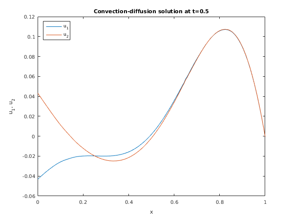
Example 1 (EX1)

This example is a simple first-order system with coupled ODEs arising from the use of the characteristic equations for the numerical boundary conditions.

The PDEs are

\begin{matrix} \frac{\partial U_{1}}{\partial t} + \frac{\partial U_{1}}{\partial x} + 2 \frac{\partial U_{2}}{\partial x} = 0, \\ \frac{\partial U_{2}}{\partial t} + 2 \frac{\partial U_{1}}{\partial x} + \frac{\partial U_{2}}{\partial x} = 0, \end{matrix}

for

x \in [0, 1]

and

t \geq 0

The PDEs have an exact solution given by

U_{1} (x, t) = f (x - 3 t) + g (x + t), U_{2} (x, t) = f (x - 3 t) - g (x + t),

where

f (z) = \exp (π z) \sin (2 π z)

g (z) = \exp (- 2 π z) \cos (2 π z)

The initial conditions are given by the exact solution.

The characteristic variables are

W_{1} = U_{1} - U_{2}

and

W_{2} = U_{1} + U_{2}

, corresponding to the characteristics given by

d x / d t = - 1

and

d x / d t = 3

respectively. Hence we require a physical boundary condition for

W_{2}

at the left-hand boundary and for

W_{1}

at the right-hand boundary (corresponding to the incoming characteristics), and a numerical boundary condition for

W_{1}

at the left-hand boundary and for

W_{2}

at the right-hand boundary (outgoing characteristics).

The physical boundary conditions are obtained from the exact solution, and the numerical boundary conditions are supplied in the form of the characteristic equations for the outgoing characteristics, that is

\frac{\partial W_{1}}{\partial t} - \frac{\partial W_{1}}{\partial x} = 0

at the left-hand boundary, and

\frac{\partial W_{2}}{\partial t} + 3 \frac{\partial W_{2}}{\partial x} = 0

at the right-hand boundary.

In order to specify these boundary conditions, two ODE variables

V_{1}

and

V_{2}

are introduced, defined by

\begin{matrix} V_{1} (t) = W_{1} (0, t) = U_{1} (0, t) - U_{2} (0, t), \\ V_{2} (t) = W_{2} (1, t) = U_{1} (1, t) + U_{2} (1, t) . \end{matrix}

The coupling points are therefore at

x = 0

and

x = 1

The numerical boundary conditions are now

{\dot{V}}_{1} - \frac{\partial W_{1}}{\partial x} = 0

at the left-hand boundary, and

{\dot{V}}_{2} + 3 \frac{\partial W_{2}}{\partial x} = 0

at the right-hand boundary.

The spatial derivatives are evaluated at the appropriate boundary points in bndary using one-sided differences (into the domain and therefore consistent with the characteristic directions).

The numerical flux is calculated using Roe's approximate Riemann solver (see Description for details), giving

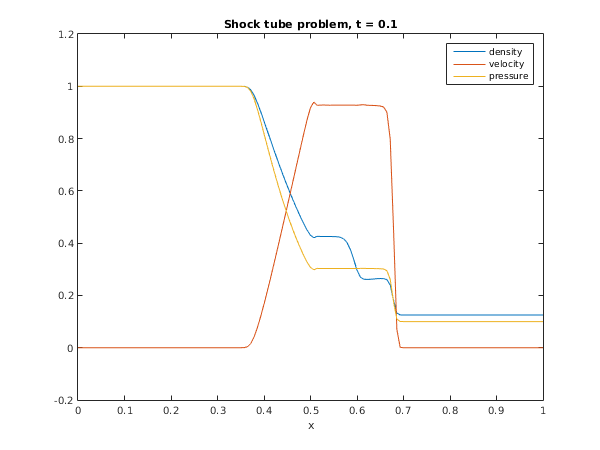
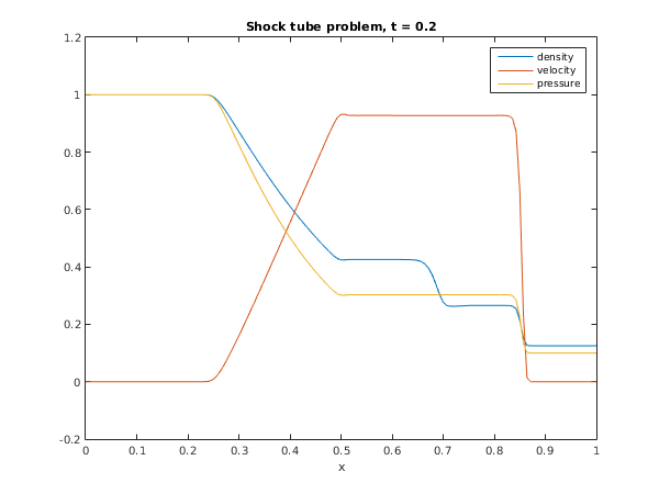
\hat{F} = \frac{1}{2} [\begin{array}{l} 3 U_{1 L} - U_{1 R} + 3 U_{2 L} + U_{2 R} \\ 3 U_{1 L} + U_{1 R} + 3 U_{2 L} - U_{2 R} \end{array}] .

Example 2 (EX2)

This example is the standard shock-tube test problem proposed by Sod (1978) for the Euler equations of gas dynamics. The problem models the flow of a gas in a long tube following the sudden breakdown of a diaphragm separating two initial gas states at different pressures and densities. There is an exact solution to this problem which is not included explicitly as the calculation is quite lengthy. The PDEs are

\begin{array}{rcl} \frac{\partial ρ}{\partial t} + \frac{\partial m}{\partial x} & = & 0, \\ \frac{\partial m}{\partial t} + \frac{\partial}{\partial x} (\frac{m^{2}}{ρ} + (γ - 1) (e - \frac{m^{2}}{2 ρ})) & = & 0, \\ \frac{\partial e}{\partial t} + \frac{\partial}{\partial x} (\frac{m e}{ρ} + \frac{m}{ρ} (γ - 1) (e - \frac{m^{2}}{2 ρ})) & = & 0, \end{array}

where

ρ

is the density;

m

is the momentum, such that

m = ρ u

, where

u

is the velocity;

e

is the specific energy; and

γ

is the (constant) ratio of specific heats. The pressure

p

is given by

p = (γ - 1) (e - \frac{ρ u^{2}}{2}) .

The solution domain is

0 \leq x \leq 1

for

0 < t \leq 0.2

, with the initial discontinuity at

x = 0.5

, and initial conditions

\begin{array}{l} ρ (x, 0) = 1, & m (x, 0) = 0, & e (x, 0) = 2.5, & for ​ x < 0.5, \\ ρ (x, 0) = 0.125, & m (x, 0) = 0, & e (x, 0) = 0.25, & for ​ x > 0.5 . \end{array}

The solution is uniform and constant at both boundaries for the spatial domain and time of integration stated, and hence the physical and numerical boundary conditions are indistinguishable and are both given by the initial conditions above. The evaluation of the numerical flux for the Euler equations is not trivial; the Roe algorithm given in Description cannot be used directly as the Jacobian is nonlinear. However, an algorithm is available using the argument-vector method (see Roe (1981)), and this is provided in the utility function nag_pde_1d_parab_euler_roe (d03pu). An alternative Approxiate Riemann Solver using Osher's scheme is provided in nag_pde_1d_parab_euler_osher (d03pv). Either nag_pde_1d_parab_euler_roe (d03pu) or nag_pde_1d_parab_euler_osher (d03pv) can be called from numflx.

Open in the MATLAB editor: d03pl_example

function d03pl_example


fprintf('d03pl example results\n\n');

fprintf('example 1\n\n');
ex1;
fprintf('\nexample 2\n\n');
ex2;



function ex1
  npde  = int64(2);
  npts  = int64(141);
  ncode = int64(2);
  neqn  = npde*npts+ncode;
  ts    = 0;
  tout  = 0.5;
  x     = zeros(npts,1);
  xi    = [0; 1];
  rtol  = [0.00025];
  atol  = [1e-05];
  itol  = int64(1);
  norm_p = '1';
  laopt  = 'S';
  algopt = zeros(30,1);
  algopt(1)  = 1;
  algopt(29) = 0.1;
  algopt(30) = 1.1;
  rsave  = zeros(11000, 1);
  isave  = zeros(15700, 1, 'int64');
  itask  = int64(1);
  itrace = int64(0);
  ind    = int64(0);

  % Initialise mesh
  dx = 1/(double(npts)-1);
  x  = [0:dx:1];

  u = exact(ts, npde, x, npts);
  u = reshape(u, [2*npts,1]);
  u(neqn-1) = u(1) - u(2);
  u(neqn)   = u(neqn-2) + u(neqn - 3);

  [ts, u, rsave, isave, ind, ifail] = ...
  d03pl( ...
         npde, ts, tout, @pdedef, @numflx1, @bndary1, u, x, ncode, ...
         @odedef, xi, rtol, atol, itol, norm_p, laopt, ...
         algopt, rsave, isave, itask, itrace, ind);
  
  xout = x(1:20:npts);
  nop = length(xout);

  uout(1, :) = u(1:20*npde:npts*npde);
  uout(2, :) = u(2:20*npde:npts*npde);

  ue = exact(tout, npde, xout, nop);

  fprintf('\n%8s%12s%12s%12s%12s\n','x','U_1','u_1','U_2','u_2');
  for i=1:nop
    fprintf('%12.4f%12.4f%12.4f%12.4f%12.4f\n', ...
            xout(i), uout(1,i), ue(1,i), uout(2,i), ue(2,i));
  end

  fig1 = figure;
  plot(x,u(1:2:npts*npde),x,u(2:2:npts*npde));
  title('Convection-diffusion solution at t=0.5');
  xlabel('x');
  ylabel('u_1, u_2');
  legend('u_1','u_2','location','NorthWest');
function ex2
  npde  = int64(3);
  npts  = int64(141);
  ncode = int64(0);
  nxi   = int64(0);
  neqn  = npde*npts+ncode;
  ts    = 0;
  x     = zeros(npts,1);
  xi    = [];
  rtol  = [0.0005];
  atol  = [0.005];
  itol  = int64(1);
  norm_p = '2';
  laopt  = 'B';
  algopt = zeros(30,1);
  algopt(1) = 2;
  algopt(6) = 2;
  algopt(7) = 2;
  algopt(13) = 0.005;
  rsave  = zeros(21000, 1);
  isave  = zeros(25700, 1, 'int64');
  itask  = int64(1);
  itrace = int64(0);
  ind    = int64(0);

  % Initialise mesh
  dx = 1/(double(npts)-1);
  x  = [0:dx:1];

  u = uvinit(x);

  for j=1:2
    tout = 0.1*j;
    [ts, u, rsave, isave, ind, ifail] = ...
    d03pl( ...
           npde, ts, tout, @pdedef, @numflx2, @bndary2, u, x, ncode, ...
           @odedef, xi, rtol, atol, itol, norm_p, laopt, ...
           algopt, rsave, isave, itask, itrace, ind,'nxi',nxi);

    density = u(1,:);
    velocity = u(2,:)./density;
    pressure = 0.4*density.*(u(3,:)./density-velocity.^2/2);
    if j==1
      fig2 = figure;
    else
      fig3 = figure;
    end
    plot(x,density,x,velocity,x,pressure);
    text = sprintf('Shock tube problem, t = %3.1f',tout);
    title(text);
    xlabel('x');
    legend('density','velocity','pressure')
  end

  nsteps = 50*((isave(1)+25)/50);
  nfuncs = 50*((isave(2)+25)/50);
  njacs = isave(3);
  niters = isave(5);
  fprintf('\n Number of time steps           (nearest 50) = %6d\n',nsteps);
  fprintf(' Number of function evaluations (nearest 50) = %6d\n',nfuncs);
  fprintf(' Number of Jacobian evaluations (nearest  1) = %6d\n',njacs);
  fprintf(' Number of iterations           (nearest  1) = %6d\n',niters);

function [g, ires] = bndary1(npde, npts, t, x, u, ncode, v, vdot, ibnd, ires)
  g = zeros(npde, 1);
  np1 = npts-1;
  if (ibnd == 0)
    ue = exact(t,npde,x(1),1);
    g(1) = u(1,1) + u(2,1) - ue(1,1) - ue(2,1);
    dudx = (u(1,2)-u(2,2)-u(1,1)+u(2,1))/(x(2)-x(1));
    g(2) = vdot(1) - dudx;
  else
    ue = exact(t,npde,x(npts),1);
    g(1) = u(1,npts) - u(2,npts) - ue(1,1) + ue(2,1);
    dudx = (u(1,npts)+u(2,npts)-u(1,np1)-u(2,np1))/(x(npts)-x(np1));
    g(2) = vdot(2) + 3*dudx;
  end

function [u] = exact(t,npde,x,npts)
  u = zeros(npde,npts);
  pi2 = 2*pi;
  for i = 1:double(npts)
   f = exp(pi*(x(i)-3*t))*sin(pi2*(x(i)-3*t));
   g = exp(-pi2*(x(i)+t))*cos(pi2*(x(i)+t));
   u(1,i) = f + g;
   u(2,i) = f - g;
  end

function [flux, ires] = numflx1(npde, t, x, ncode, v, uleft, uright, ires)
  flux = zeros(npde, 1);
  flux(1) = (3*uleft(1)-uright(1)+3*uleft(2)+uright(2))/2;
  flux(2) = (3*uleft(1)+uright(1)+3*uleft(2)-uright(2))/2;

function [r, ires] = odedef(npde, t, ncode, v, vdot, nxi, xi, ucp, ucpx, ...
                            ucpt, ires)
  r = zeros(ncode, 1);
  if (ires ~= -1)
    r(1) = v(1) - ucp(1,1) + ucp(2,1);
    r(2) = v(2) - ucp(1,2) - ucp(2,2);
  end

function [p, c, d, s, ires] = pdedef(npde, t, x, u, ux, ncode, v, vdot, ires)
  p = eye(npde);
  c = ones(npde,1);
  d = zeros(npde, 1);
  s = d;

function [g, ires] = bndary2(npde, npts, t, x, u, ncode, v, vdot, ibnd, ires)
  
  if (ibnd == 0)
    g(1) = u(1,1) - 1;
    g(2) = u(2,1);
    g(3) = u(3,1) - 2.5;
  else
    g(1) = u(1,npts) - 1/8;
    g(2) = u(2,npts);
    g(3) = u(3,npts) - 1/4;
  end

function [flux, ires] = numflx2(npde, t, x, ncode, v, uleft, uright, ires)

  % Use Rho scheme rputine d03pu (Osher scheme d03pv is an alternative)
  gamma = 1.4;
  [flux, ifail] = d03pu( ...
                         uleft, uright, gamma);

function [u] = uvinit(x)
  n = size(x,2);
  u = zeros(3,n);
  for i = 1:n
    if x(i)<1/2
      u(1,i) = 1;
      u(3,i) = 2.5;
    elseif x(i)== 1/2
      u(1,i) = (1+1/8)/2;
      u(3,i) = (2.5+1/4)/2;
    else
      u(1,i) = 1/8;
      u(3,i) = 1/4;
    end
  end

d03pl example results

example 1


       x         U_1         u_1         U_2         u_2
      0.0000     -0.0432     -0.0432      0.0432      0.0432
      0.1429     -0.0221     -0.0220      0.0001     -0.0000
      0.2857     -0.0199     -0.0199     -0.0231     -0.0231
      0.4286     -0.0123     -0.0123     -0.0175     -0.0176
      0.5714      0.0247      0.0245      0.0226      0.0224
      0.7143      0.0832      0.0827      0.0830      0.0825
      0.8571      0.1041      0.1036      0.1043      0.1039
      1.0000     -0.0007     -0.0001     -0.0005      0.0001

example 2


 Number of time steps           (nearest 50) =    200
 Number of function evaluations (nearest 50) =    450
 Number of Jacobian evaluations (nearest  1) =      1
 Number of iterations           (nearest  1) =      2

PDF version (NAG web site, 64-bit version, 64-bit version)

Chapter Contents

Chapter Introduction

NAG Toolbox