PDF version (NAG web site
, 64-bit version, 64-bit version)
NAG Toolbox: nag_tsa_uni_autocorr (g13ab)
Purpose
nag_tsa_uni_autocorr (g13ab) computes the sample autocorrelation function of a time series. It also computes the sample mean, the sample variance and a statistic which may be used to test the hypothesis that the true autocorrelation function is zero.
Syntax
Description
The data consists of observations , for from a time series.
The quantities calculated are
| (a) |
The sample mean
|
| (b) |
The sample variance (for )
|
| (c) |
The sample autocorrelation coefficients of lags , where is a user-specified maximum lag, and , .
The coefficient of lag is defined as
See page 496 of Box and Jenkins (1976) for further details. |
| (d) |
A test statistic defined as
which can be used to test the hypothesis that the true autocorrelation function is identically zero.
If is large and is much smaller than , stat has a distribution under the hypothesis of a zero autocorrelation function. Values of stat in the upper tail of the distribution provide evidence against the hypothesis; nag_stat_prob_chisq (g01ec) can be used to compute the tail probability. Section 8.2.2 of Box and Jenkins (1976) provides further details of the use of stat. |
References
Box G E P and Jenkins G M (1976) Time Series Analysis: Forecasting and Control (Revised Edition) Holden–Day
Parameters
Compulsory Input Parameters
- 1:
– double array
-
The time series,
, for .
- 2:
– int64int32nag_int scalar
-
, the number of lags for which the autocorrelations are required. The lags range from to and do not include zero.
Constraint:
.
Optional Input Parameters
- 1:
– int64int32nag_int scalar
-
Default:
the dimension of the array
x.
, the number of values in the time series.
Constraint:
.
Output Parameters
- 1:
– double scalar
-
The sample mean of the input time series.
- 2:
– double scalar
-
The sample variance of the input time series.
- 3:
– double array
-
The sample autocorrelation coefficient relating to lag
, for .
- 4:
– double scalar
-
The statistic used to test the hypothesis that the true autocorrelation function of the time series is identically zero.
- 5:
– int64int32nag_int scalar
unless the function detects an error (see
Error Indicators and Warnings).
Error Indicators and Warnings
Errors or warnings detected by the function:
Cases prefixed with W are classified as warnings and
do not generate an error of type NAG:error_n. See nag_issue_warnings.
-
-
| On entry, | , |
| or | , |
| or | . |
- W
-
On entry, all values of
x are practically identical, giving zero variance. In this case
r and
stat are undefined on exit.
-
An unexpected error has been triggered by this routine. Please
contact
NAG.
-
Your licence key may have expired or may not have been installed correctly.
-
Dynamic memory allocation failed.
Accuracy
The computations are believed to be stable.
Further Comments
If , or then the autocorrelations are calculated directly and the time taken by nag_tsa_uni_autocorr (g13ab) is approximately proportional to , otherwise the autocorrelations are calculated by utilizing fast fourier transforms (FFTs) and the time taken is approximately proportional to . If FFTs are used then nag_tsa_uni_autocorr (g13ab) internally allocates approximately real elements.
If the input series for
nag_tsa_uni_autocorr (g13ab) was generated by differencing using
nag_tsa_uni_diff (g13aa), ensure that only the differenced values are input to
nag_tsa_uni_autocorr (g13ab), and not the reconstituting information.
Example
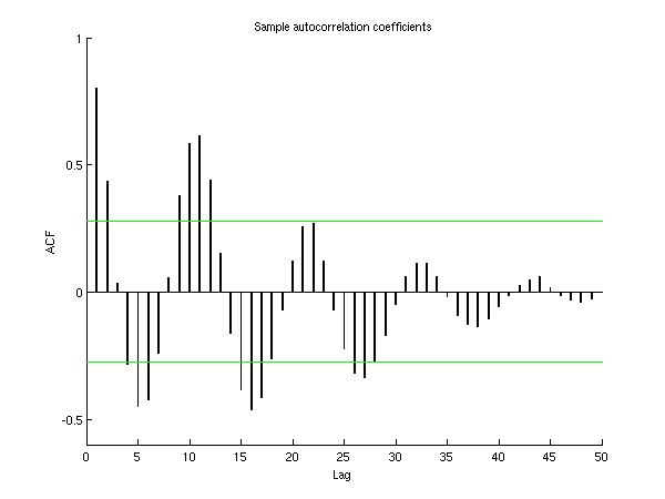
In the example below, a set of values of sunspot counts is used as input. The first autocorrelations are computed.
Open in the MATLAB editor:
g13ab_example
function g13ab_example
fprintf('g13ab example results\n\n');
x = [ 5; 11; 16; 23; 36; 58; 29; 20; 10; 8;
3; 0; 0; 2; 11; 27; 47; 63; 60; 39;
28; 26; 22; 11; 21; 40; 78; 122; 103; 73;
47; 35; 11; 5; 16; 34; 70; 81; 111; 101;
73; 40; 20; 16; 5; 11; 22; 40; 60; 80.9];
nk = int64(10);
[xm, xv, r, stat, ifail] = g13ab( ...
x, nk);
fprintf('The first %4d coefficients are required\n',nk);
fprintf('The input array has sample mean %12.4f\n', xm);
fprintf('The input array has sample variance %12.4f\n', xv);
fprintf('The sample autocorrelation coefficients are\n\n');
fprintf(' Lag Coeff Lag Coeff\n');
ivar = double([1:nk]);
fprintf('%6d%10.4f%8d%10.4f\n',[ivar; r(1:nk)']);
fprintf('\nThe value of stat is %12.4f\n', stat);
nk = int64(numel(x)-1);
[xm, xv, r, stat, ifail] = g13ab( ...
x, nk);
fig1 = figure;
refline = 1.96/sqrt(numel(x));
hold on
h = bar(r,0.1);
h.FaceColor = [1 0 0];
h.EdgeColor = [1 0 0];
h.ShowBaseLine = 'off';
plot([0 nk+1],[refline refline],'green');
plot([0 nk+1],[-refline -refline],'green');
axis([0 50 -0.6 1]);
ax = gca;
ax.YTick = [-0.6:0.2:1];
ax.XTick = [0:10:50];
xlabel('Lag');
ylabel('ACF');
title('Sample autocorrelation coefficients');
hold off
g13ab example results

The first   10 coefficients are required
The input array has sample mean          37.4180
The input array has sample variance    1002.0301
The sample autocorrelation coefficients are

   Lag    Coeff      Lag    Coeff
     1    0.8004       2    0.4355
     3    0.0328       4   -0.2835
     5   -0.4505       6   -0.4242
     7   -0.2419       8    0.0550
     9    0.3783      10    0.5857

The value of stat is      92.1231
This plot shows the autocorrelations for all possible lag values. Reference lines are given at .
PDF version (NAG web site
, 64-bit version, 64-bit version)
© The Numerical Algorithms Group Ltd, Oxford, UK. 2009–2015
