nag_fit_1dcheb_eval2 (e02ak) evaluates a polynomial from its Chebyshev series representation, allowing an arbitrary index increment for accessing the array of coefficients.

Syntax

[result, ifail] = e02ak(n, xmin, xmax, a, ia1, x)

[result, ifail] = nag_fit_1dcheb_eval2(n, xmin, xmax, a, ia1, x)

Description

If supplied with the coefficients

a_{i}

, for

i = 0, 1, \dots, n

, of a polynomial

p (\bar{x})

of degree

n

, where

p (\bar{x}) = \frac{1}{2} a_{0} + a_{1} T_{1} (\bar{x}) + \dots + a_{n} T_{n} (\bar{x}),

nag_fit_1dcheb_eval2 (e02ak) returns the value of

p (\bar{x})

at a user-specified value of the variable

x

. Here

T_{j} (\bar{x})

denotes the Chebyshev polynomial of the first kind of degree

j

with argument

\bar{x}

. It is assumed that the independent variable

\bar{x}

in the interval

[- 1, + 1]

was obtained from your original variable

x

in the interval

[x_{\min}, x_{\max}]

by the linear transformation

\bar{x} = \frac{2 x - (x_{\max} + x_{\min})}{x_{\max} - x_{\min}} .

The coefficients

a_{i}

may be supplied in the array a, with any increment between the indices of array elements which contain successive coefficients. This enables the function to be used in surface fitting and other applications, in which the array might have two or more dimensions.

The method employed is based on the three-term recurrence relation due to Clenshaw (see Clenshaw (1955)), with modifications due to Reinsch and Gentleman (see Gentleman (1969)). For further details of the algorithm and its use see Cox (1973) and Cox and Hayes (1973).

References

Clenshaw C W (1955) A note on the summation of Chebyshev series Math. Tables Aids Comput. 9 118–120

Cox M G (1973) A data-fitting package for the non-specialist user NPL Report NAC 40 National Physical Laboratory

Cox M G and Hayes J G (1973) Curve fitting: a guide and suite of algorithms for the non-specialist user NPL Report NAC26 National Physical Laboratory

Gentleman W M (1969) An error analysis of Goertzel's (Watt's) method for computing Fourier coefficients Comput. J. 12 160–165

Parameters

Compulsory Input Parameters

1: $n$ – int64int32nag_int scalar

n

, the degree of the given polynomial

p (\bar{x})

Constraint:

n \geq 0

2: $xmin$ – double scalar

3: $xmax$ – double scalar

The lower and upper end points respectively of the interval

[x_{\min}, x_{\max}]

. The Chebyshev series representation is in terms of the normalized variable

\bar{x}

, where

\bar{x} = \frac{2 x - (x_{\max} + x_{\min})}{x_{\max} - x_{\min}} .

Constraint:

xmin < xmax

4: $a (la)$ – double array

la, the dimension of the array, must satisfy the constraint

la \geq (np1 - 1) \times ia1 + 1

The Chebyshev coefficients of the polynomial

p (\bar{x})

. Specifically, element

i \times ia1 + 1

must contain the coefficient

a_{i}

, for

i = 0, 1, \dots, n

. Only these

n + 1

elements will be accessed.

5: $ia1$ – int64int32nag_int scalar

The index increment of a. Most frequently, the Chebyshev coefficients are stored in adjacent elements of a, and ia1 must be set to

1

. However, if, for example, they are stored in

a (1), a (4), a (7), \dots

, then the value of ia1 must be

3

Constraint:

ia1 \geq 1

6: $x$ – double scalar

The argument

x

at which the polynomial is to be evaluated.

Constraint:

xmin \leq x \leq xmax

Optional Input Parameters

None.

Output Parameters

1: $result$ – double scalar: The value of the polynomial $p (\bar{x})$ .
2: $ifail$ – int64int32nag_int scalar: $ifail = 0$ unless the function detects an error (see Error Indicators and Warnings).

Error Indicators and Warnings

Errors or warnings detected by the function:

$ifail = 1$

On entry,	$np1 < 1$ ,
or	$ia1 < 1$ ,
or	$la \leq (np1 - 1) \times ia1$ ,
or	$xmin \geq xmax$ .

$ifail = 2$: x does not satisfy the restriction $xmin \leq x \leq xmax$ .

$ifail = - 99$: An unexpected error has been triggered by this routine. Please contact NAG.

$ifail = - 399$: Your licence key may have expired or may not have been installed correctly.

$ifail = - 999$: Dynamic memory allocation failed.

Accuracy

The rounding errors are such that the computed value of the polynomial is exact for a slightly perturbed set of coefficients

a_{i} + δ a_{i}

. The ratio of the sum of the absolute values of the

δ a_{i}

to the sum of the absolute values of the

a_{i}

is less than a small multiple of

(n + 1) \times machine precision

Further Comments

The time taken is approximately proportional to

n + 1

Example

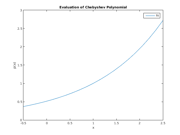
Suppose a polynomial has been computed in Chebyshev series form to fit data over the interval

[- 0.5, 2.5]

. The following program evaluates the polynomial at

4

equally spaced points over the interval. (For the purposes of this example, xmin, xmax and the Chebyshev coefficients are supplied . Normally a program would first read in or generate data and compute the fitted polynomial.)

Open in the MATLAB editor: e02ak_example

function e02ak_example


fprintf('e02ak example results\n\n');

xmin = -0.5; xmax = 2.5;
a = [2.53213  1.13032  0.2715  0.04434   0.00547   0.00054  4e-05];

n = int64(6);
ia1 = int64(1);

% Evaluate polynomial from coefficients a at x
m = 21;
dx =  (xmax-xmin)/(m-1);
x = [xmin:dx:xmax];

for i = 1:m
  [fit(i), ifail] = e02ak( ...
                             n, xmin, xmax, a, ia1, x(i));
end

sol = [x; fit];
fprintf('     x           p(x)\n');
fprintf('%9.4f    %9.4f\n',sol(1:2,1:5:21));

fig1 = figure;
plot(x,fit);
title('Evaluation of Chebyshev Polynomial');
xlabel('x');
ylabel('p(x)');
legend('fit','exp(x)');

e02ak example results

     x           p(x)
  -0.5000       0.3679
   0.2500       0.6065
   1.0000       1.0000
   1.7500       1.6487
   2.5000       2.7183

PDF version (NAG web site, 64-bit version, 64-bit version)

Chapter Contents

Chapter Introduction

NAG Toolbox