PDF version (NAG web site
, 64-bit version, 64-bit version)
NAG Toolbox: nag_interp_2d_scat (e01sa)
Purpose
nag_interp_2d_scat (e01sa) generates a two-dimensional surface interpolating a set of scattered data points, using the method of Renka and Cline.
Syntax
Description
nag_interp_2d_scat (e01sa) constructs an interpolating surface through a set of scattered data points , for , using a method due to Renka and Cline. In the plane, the data points must be distinct. The constructed surface is continuous and has continuous first derivatives.
The method involves firstly creating a triangulation with all the
data points as nodes, the triangulation being as nearly equiangular as possible (see
Cline and Renka (1984)). Then gradients in the
- and
-directions are estimated at node
, for
,
as the partial derivatives of a quadratic function of
and
which interpolates the data value
,
and which fits the data values at nearby nodes (those within a certain distance chosen by the algorithm) in a weighted least squares sense. The weights are chosen such that closer nodes have more influence than more distant nodes on derivative estimates at node
. The computed partial derivatives, with the
values, at the three nodes of each triangle define a piecewise polynomial surface of a certain form which is the interpolant on that triangle. See
Renka and Cline (1984) for more detailed information on the algorithm,
a development of that by
Lawson (1977). The code is derived from
Renka (1984).
The interpolant
can subsequently be evaluated at any point
inside or outside the domain of the data by a call to
nag_interp_2d_scat_eval (e01sb).
Points outside the domain are evaluated by extrapolation.
References
Cline A K and Renka R L (1984) A storage-efficient method for construction of a Thiessen triangulation Rocky Mountain J. Math. 14 119–139
Lawson C L (1977) Software for surface interpolation Mathematical Software III (ed J R Rice) 161–194 Academic Press
Renka R L (1984) Algorithm 624: triangulation and interpolation of arbitrarily distributed points in the plane ACM Trans. Math. Software 10 440–442
Renka R L and Cline A K (1984) A triangle-based interpolation method Rocky Mountain J. Math. 14 223–237
Parameters
Compulsory Input Parameters
- 1:
– double array
- 2:
– double array
- 3:
– double array
-
The coordinates of the
th data point, for
. The data points are accepted in any order, but see
Further Comments.
Constraint:
the nodes must not all be collinear, and each node must be unique.
Optional Input Parameters
- 1:
– int64int32nag_int scalar
-
Default:
the dimension of the arrays
x,
y,
f. (An error is raised if these dimensions are not equal.)
, the number of data points.
Constraint:
.
Output Parameters
- 1:
– int64int32nag_int array
-
A data structure defining the computed triangulation, in a form suitable for passing to
nag_interp_2d_scat_eval (e01sb).
- 2:
– double array
-
The estimated partial derivatives at the nodes, in a form suitable for passing to
nag_interp_2d_scat_eval (e01sb). The derivatives at node
with respect to
and
are contained in
and
respectively, for
.
- 3:
– int64int32nag_int scalar
unless the function detects an error (see
Error Indicators and Warnings).
Error Indicators and Warnings
Errors or warnings detected by the function:
-
-
-
-
| On entry, | all the (x,y) pairs are collinear. |
-
-
| On entry, | for some . |
-
An unexpected error has been triggered by this routine. Please
contact
NAG.
-
Your licence key may have expired or may not have been installed correctly.
-
Dynamic memory allocation failed.
Accuracy
On successful exit, the computational errors should be negligible in most situations but you should always check the computed surface for acceptability, by drawing contours for instance. The surface always interpolates the input data exactly.
Further Comments
The time taken for a call of
nag_interp_2d_scat (e01sa) is approximately proportional to the number of data points,
. The function is more efficient if, before entry, the values in
x,
y and
f are arranged so that the
x array is in ascending order.
Example
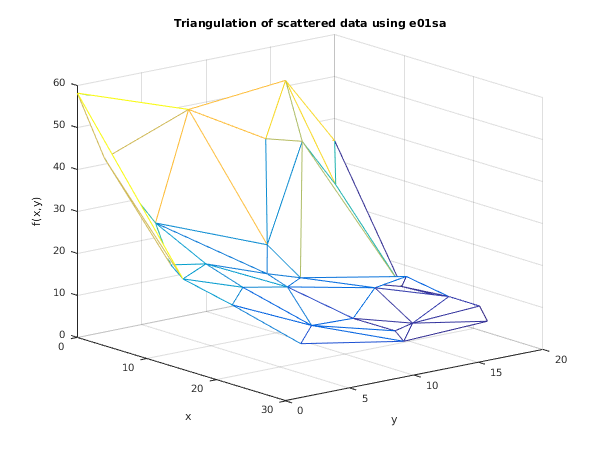
This example reads in a set of
data points and calls
nag_interp_2d_scat (e01sa)
to construct an interpolating surface. It then calls
nag_interp_2d_scat_eval (e01sb)
to evaluate the interpolant at a sample of points on a rectangular grid.
Note that this example is not typical of a realistic problem: the number of data points would normally be larger, and the interpolant would need to be evaluated on a finer grid to obtain an accurate plot, say.
Open in the MATLAB editor:
e01sa_example
function e01sa_example
fprintf('e01sa example results\n\n');
x = [11.16; 12.85; 19.85; 19.72; 15.91; 0.00; 20.87; 3.45; 14.26; ...
17.43; 22.80; 7.58; 25.00; 0.00; 9.66; 5.22; 17.25; 25.00; ...
12.13; 22.23; 11.52; 15.20; 7.54; 17.32; 2.14; 0.51; 22.69; ...
5.47; 21.67; 3.31];
y = [ 1.24; 3.06; 10.72; 1.39; 7.74; 20.00; 20.00; 12.78; 17.87; ...
3.46; 12.39; 1.98; 11.87; 0.00; 20.00; 14.66; 19.57; 3.87; ...
10.79; 6.21; 8.53; 0.00; 10.69; 13.78; 15.03; 8.37; 19.63; ...
17.13; 14.36; 0.33];
f = [22.15; 22.11; 7.97; 16.83; 15.30; 34.60; 5.74; 41.24; 10.74; ...
18.60; 5.47; 29.87; 4.40; 58.20; 4.73; 40.36; 6.43; 8.74; ...
13.71; 10.25; 15.74; 21.60; 19.31; 12.11; 53.10; 49.43; 3.25; ...
28.63; 5.52; 44.08];
[triang,grads,ifail] = e01sa(x,y,f);
n = size(x,1);
[tri,k] = triang2tri(triang,n);
fprintf('Number of triangles in triangulation = %d\n\n',k);
fig1 = figure;
trimesh(tri(1:k,1:3),x,y,f);
xlabel('x');
ylabel('y');
zlabel('f(x,y)')
title('Triangulation of scattered data using e01sa');
view(51,18);
px = [3:3:21];
py = [2:3:17];
for i = 1:6
for j = 1:7
[pf(i,j), ifail] = e01sb( ...
x, y, f, triang, grads, px(j), py(i));
end
end
matrix = 'General';
diag = 'Non-unit';
format = 'F7.2';
mtitl = 'Spline evaluated on a regular mesh (x across, y down):';
chlab = 'Character';
rlabs = cellstr(num2str(py'));
clabs = cellstr(num2str(px'));
ncols = int64(80);
indent = int64(0);
[ifail] = x04cb( ...
matrix, diag, pf, format, mtitl, chlab, ...
rlabs, chlab, clabs, ncols, indent);
function [tri,k] = triang2tri(triang,n)
max_t = int64(2*n-5);
tri = int64(zeros(max_t,3));
iend = int64(0);
k = iend;
t = int64([0;0;0]);
for i = 1:n
ibeg = iend + 1;
iend = triang(6*n+i);
t(1) = i;
t(2) = triang(ibeg);
ibeg = ibeg + 1;
for j = ibeg:iend
t(3) = triang(j);
if t(3)>0
if t(2)>i || t(3)>i
k = k + 1;
tri(k,1:3) = t(1:3);
end
t(2) = t(3);
end
end
end
e01sa example results

Number of triangles in triangulation = 88

 Spline evaluated on a regular mesh (x across, y down):
          3      6      9     12     15     18     21
  2   43.52  33.91  26.59  22.23  21.15  18.67  14.88
  5   40.49  29.26  22.51  20.72  19.30  16.72  12.87
  8   37.90  23.97  16.79  16.43  15.46  13.02   9.30
 11   38.55  25.25  16.72  13.83  13.08  10.71   6.88
 14   47.61  36.66  22.87  14.02  13.44  11.20   6.46
 17   41.25  27.62  18.03  12.29  11.68   9.09   5.37
PDF version (NAG web site
, 64-bit version, 64-bit version)
© The Numerical Algorithms Group Ltd, Oxford, UK. 2009–2015
