PDF version (NAG web site
, 64-bit version, 64-bit version)
NAG Toolbox: nag_ode_bvp_shoot_genpar (d02hb)
Purpose
nag_ode_bvp_shoot_genpar (d02hb) solves a two-point boundary value problem for a system of ordinary differential equations, using initial value techniques and Newton iteration; it generalizes function
nag_ode_bvp_shoot_bval (d02ha) to include the case where parameters other than boundary values are to be determined.
Syntax
[
p,
soln,
w,
ifail] = d02hb(
p,
pe,
e,
m1,
fcn,
bc,
range, 'n1',
n1, 'n',
n)
[
p,
soln,
w,
ifail] = nag_ode_bvp_shoot_genpar(
p,
pe,
e,
m1,
fcn,
bc,
range, 'n1',
n1, 'n',
n)
Description
nag_ode_bvp_shoot_genpar (d02hb) solves a two-point boundary value problem by determining the unknown parameters
of the problem. These parameters may be, but need not be, boundary values; they may include eigenvalue parameters in the coefficients of the differential equations, length of the range of integration, etc. The notation and methods used are similar to those of
nag_ode_bvp_shoot_bval (d02ha) and you are advised to study this first. (The parameters
correspond precisely to the unknown boundary conditions in
nag_ode_bvp_shoot_bval (d02ha).) It is assumed that we have a system of
first-order ordinary differential equations of the form:
and that the derivatives
are evaluated by
fcn. The system, including the boundary conditions given by
bc and the range of integration given by
range, involves the
unknown parameters
which are to be determined, and for which initial estimates must be supplied. The number of unknown parameters
must not exceed the number of equations
. If
, we assume that
equations of the system are not involved in the matching process. These are usually referred to as ‘driving equations’; they are independent of the parameters and of the solutions of the other
equations. In numbering the equations for
fcn, the driving equations must be put
first.
The estimated values of the parameters are corrected by a form of Newton iteration. The Newton correction on each iteration is calculated using a Jacobian matrix whose th element depends on the derivative of the th component of the solution, , with respect to the th parameter, . This matrix is calculated by a simple numerical differentiation technique which requires evaluations of the differential system.
If the argument
ifail is set appropriately, the function automatically prints messages to inform you of the flow of the calculation. These messages are discussed in detail in
Further Comments.
nag_ode_bvp_shoot_genpar (d02hb) is a simplified version of
nag_ode_bvp_shoot_genpar_algeq (d02sa) which is described in detail in
Gladwell (1979).
References
Gladwell I (1979) The development of the boundary value codes in the ordinary differential equations chapter of the NAG Library Codes for Boundary Value Problems in Ordinary Differential Equations. Lecture Notes in Computer Science (eds B Childs, M Scott, J W Daniel, E Denman and P Nelson) 76 Springer–Verlag
Parameters
You are strongly recommended to read
Description and
Further Comments in conjunction with this section.
Compulsory Input Parameters
- 1:
– double array
-
An estimate for the
th argument, , for .
- 2:
– double array
-
The elements of
pe must be given small positive values. The element
is used
| (i) |
in the convergence test on the th argument in the Newton iteration, and |
| (ii) |
in perturbing the th argument when approximating the derivatives of the components of the solution with respect to this argument for use in the Newton iteration. |
The elements
should not be chosen too small. They should usually be several orders of magnitude larger than
machine precision.
Constraint:
, for .
- 3:
– double array
-
The elements of
e must be given positive values. The element
is used in the bound on the local error in the
th component of the solution
during integration.
The elements
should not be chosen too small. They should usually be several orders of magnitude larger than
machine precision.
Constraint:
, for .
- 4:
– int64int32nag_int scalar
-
A value which controls exit values.
- The final solution is not calculated.
- The final values of the solution at interval (length of range)/ are calculated and stored sequentially in the array soln starting with the values of the solutions evaluated at the first end point (see range) stored in the first column of soln.
Constraint:
.
- 5:
– function handle or string containing name of m-file
-
fcn must evaluate the functions
(i.e., the derivatives
), for
, at a general point
.
[f] = fcn(x, y, p)
Input Parameters
- 1:
– double scalar
-
, the value of the argument.
- 2:
– double array
-
, for , the value of the argument.
- 3:
– double array
-
The current estimate of the argument
, for .
Output Parameters
- 1:
– double array
-
The value of
, for
. The
may depend upon the parameters
, for
. If there are any driving equations (see
Description) then these must be numbered first in the ordering of the components of
f in
fcn.
- 6:
– function handle or string containing name of m-file
-
bc must place in
g1 and
g2 the boundary conditions at
and
respectively (see
range).
[g1, g2] = bc(p)
Input Parameters
- 1:
– double array
-
An estimate of the argument
, for .
Output Parameters
- 1:
– double array
-
The value of
, (where this may be a known value or a function of the parameters , for and ).
- 2:
– double array
-
The value of
, for
, (where these may be known values or functions of the parameters
, for
). If
, so that there are some driving equations, then the first
values of
g2 need not be set since they are never used.
- 7:
– function handle or string containing name of m-file
-
range must evaluate the boundary points
and
, each of which may depend on the arguments
. The integrations in the shooting method are always from
to
.
[a, b] = range(p)
Input Parameters
- 1:
– double array
-
The current estimate of the
th argument, , for .
Output Parameters
- 1:
– double scalar
-
, one of the boundary points.
- 2:
– double scalar
-
The second boundary point,
. Note that
forces the direction of integration to be that of increasing
. If
a and
b are interchanged the direction of integration is reversed.
Optional Input Parameters
- 1:
– int64int32nag_int scalar
-
Default:
the dimension of the arrays
p,
pe. (An error is raised if these dimensions are not equal.)
, the number of arguments.
Constraint:
.
- 2:
– int64int32nag_int scalar
-
Default:
the dimension of the array
e.
, the total number of differential equations.
Constraint:
.
Output Parameters
- 1:
– double array
-
The corrected value for the th argument, unless an error has occurred, when it contains the last calculated value of the argument.
- 2:
– double array
-
The solution when .
- 3:
– double array
-
.
With
,
,
or
(see
Error Indicators and Warnings),
, for
, contains the solution at the point
when the error occurred.
contains
.
- 4:
– int64int32nag_int scalar
unless the function detects an error (see
Error Indicators and Warnings).
Error Indicators and Warnings
Errors or warnings detected by the function:
-
-
One or more of the arguments
n,
n1,
m1,
sdw,
e or
pe is incorrectly set.
-
-
The step length for the integration became too short whilst calculating the residual (see
Further Comments).
-
-
No initial step length could be chosen for the integration whilst calculating the residual.
Note: or
can occur due to choosing too small a value for
e or due to choosing the wrong direction of integration. Try varying
e and interchanging
and
. These error exits can also occur for very poor initial choices of the parameters in the array
p and, in extreme cases, because
nag_ode_bvp_shoot_genpar (d02hb) cannot be used to solve the problem posed.
-
-
As for but the error occurred when calculating the Jacobian.
-
-
As for but the error occurred when calculating the Jacobian.
-
-
The calculated Jacobian has an insignificant column. This can occur because a parameter is incorrectly entered when posing the problem.
Note: ,
or
usually indicate a badly scaled problem. You may vary the size of
pe. Otherwise the use of the more general
nag_ode_bvp_shoot_genpar_algeq (d02sa) which affords more control over the calculations is advised.
-
-
The linear algebra function used (
nag_lapack_dgesvd (f08kb)) has failed. This error exit should not occur and can be avoided by changing the initial estimates
.
-
-
The Newton iteration has failed to converge. This can indicate a poor initial choice of parameters or a very difficult problem. Consider varying the elements if the residuals are small in the monitoring output. If the residuals are large, try varying the initial parameters .
-
-
-
-
-
-
Indicates that a serious error has occurred. Check all array subscripts and function argument lists in the call to nag_ode_bvp_shoot_genpar (d02hb). Seek expert help.
-
An unexpected error has been triggered by this routine. Please
contact
NAG.
-
Your licence key may have expired or may not have been installed correctly.
-
Dynamic memory allocation failed.
Accuracy
If the process converges, the accuracy to which the unknown parameters are determined is usually close to that specified by you; the solution, if requested, may be determined to a required accuracy by varying
e.
Further Comments
The time taken by nag_ode_bvp_shoot_genpar (d02hb) depends on the complexity of the system, and on the number of iterations required. In practice, integration of the differential equations is by far the most costly process involved.
Wherever they occur in the function, the error arguments contained in the arrays
e and
pe are used in ‘mixed’ form; that is
always occurs in expressions of the form
and
always occurs in expressions of the form
Though not ideal for every application, it is expected that this mixture of absolute and relative error testing will be adequate for most purposes.
You may determine a suitable direction of integration
to
and suitable values for
by integrations with
nag_ode_ivp_rkts_range (d02pe). The best direction of integration is usually the direction of decreasing solutions.
You are strongly recommended to set
ifail to obtain self-explanatory error messages, and also monitoring information about the course of the computation. You may select the channel numbers on which this output is to appear by calls of
nag_file_set_unit_error (x04aa) (for error messages) or
nag_file_set_unit_advisory (x04ab) (for monitoring information) – see
Example for an example. Otherwise the default channel numbers will be used. The monitoring information produced at each iteration includes the current parameter values, the residuals and
-norms: a basic norm and a current norm. At each iteration the aim is to find parameter values which make the current norm less than the basic norm. Both these norms should tend to zero as should the residuals. (They would all be zero if the exact parameters were used as input.) For more details, in particular about the other monitoring information printed, you are advised to consult the specification of
nag_ode_bvp_shoot_genpar_algeq (d02sa), and especially the description of the argument
monit there.
The computing time for integrating the differential equations can sometimes depend critically on the quality of the initial estimates for the parameters
. If it seems that too much computing time is required and, in particular, if the values of the residuals printed by the monitoring function are much larger than the expected values of the solution at
, then the coding of
fcn,
bc and
range should be checked for errors. If no errors can be found, an independent attempt should be made to improve the initial estimates for
.
The function can be used to solve a very wide range of problems, for example:
| (a) |
eigenvalue problems, including problems where the eigenvalue occurs in the boundary conditions; |
| (b) |
problems where the differential equations depend on some parameters which are to be determined so as to satisfy certain boundary conditions (see Example 2 in Example); |
| (c) |
problems where one of the end points of the range of integration is to be determined as the point where a variable takes a particular value (see Example 2 in Example); |
| (d) |
singular problems and problems on infinite ranges of integration where the values of the solution at or or both are determined by a power series or an asymptotic expansion (or a more complicated expression) and where some of the coefficients in the expression are to be determined (see Example 1 in Example); and |
| (e) |
differential equations with certain terms defined by other independent (driving) differential equations. |
Example
For this function two examples are presented. There is a single example program for nag_ode_bvp_shoot_genpar (d02hb), with a main program and the code to solve the two example problems given in Example 1 (EX1) and Example 2 (EX2).
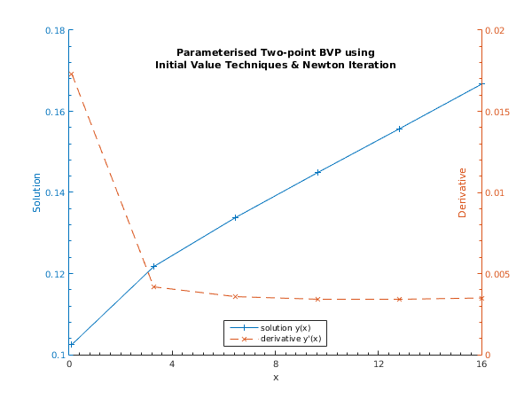
Example 1 (EX1)
This example finds the solution of the differential equation
on the range
, with boundary conditions
and
. We cannot use the differential equation at
because it is singular, so we take a truncated power series expansion
near the origin where
is one of the parameters to be determined. We choose the interval as
and setting
, we can determine all the boundary conditions. We take
. We write
,
, and estimate
,
. Note the call to
nag_file_set_unit_advisory (x04ab) before the call to
nag_ode_bvp_shoot_genpar (d02hb).
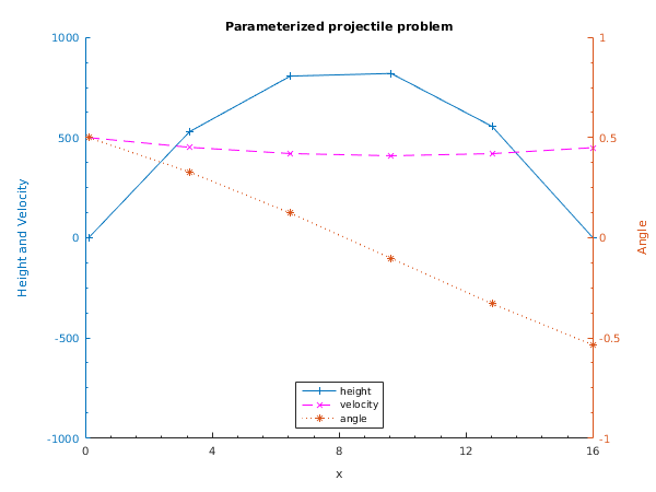
Example 2 (EX2)
This example finds the gravitational constant and the range over which a projectile must be fired to hit the target with a given velocity.
The differential equations are
on the range
, with boundary conditions
We write
,
,
. We estimate
,
and
(though this last estimate is not important).
Open in the MATLAB editor:
d02hb_example
function d02hb_example
fprintf('d02hb example results\n\n');
n = int64(2);
n1 = int64(2);
p = [0.2;0];
pe = [1e-05;0.001];
e = [0.0001;0.0001];
m1 = int64(6);
marray = zeros(1,m1);
fprintf('d02hb example program results \n');
fprintf('\nCase 1 \n\n');
[pOut1, solnOut1, w1, ifail] = ...
d02hb(...
p, pe, e, m1, @fcn1, @bc1, @range1, 'n1', n1, 'n', n);
fprintf('Final parameters \n')
fprintf(' %1.3e ',pOut1);
fprintf('\n\n Final solution \n')
fprintf('X-value Components of solution \n')
[x0, x1] = range1(p);
h = (x1-x0)/double(m1-1);
for i = 1:m1;
m = x0 + double(i-1)*h;
fprintf('%7.3f', m);
fprintf('%12.4f',solnOut1(1:n,i));
fprintf('\n');
marray(i) = m;
end
fprintf('\nCase 2 \n\n');
n = int64(3);
n1 = n;
p = [32;6000;0.54];
pe = [1e-05;1e-4;1e-4];
e = [1e-2;1e-2;1e-2];
m1 = int64(6);
qarray = zeros(1,m1);
[pOut2, solnOut2, w2, ifail] = ...
d02hb(...
p, pe, e, int64(m1), @fcn2, @bc2, @range2, 'n1', n1, 'n', n);
fprintf('Final parameters \n')
fprintf(' %1.3e ',pOut2);
fprintf('\n\n Final solution \n')
fprintf(' X-value Components of solution \n')
[x0, x1] = range2(pOut2);
h = (x1-x0)/double(m1-1);
for i = 1:m1;
q = x0 + double(i-1)*h;
fprintf('%6.0f', q);
fprintf('%12.4f',solnOut2(1:n,i));
fprintf('\n');
qarray(i) = q;
end
fig1 = figure;
display_plot(marray, solnOut1, 'Derivative');
fig2 = figure;
display_plot(marray, solnOut2, 'Angle');
function [g1, g2] = bc1(p)
z=0.1;
g1(1) = 0.1+p(1)*sqrt(z)*0.1+0.01*z;
g1(2) = p(1)*0.05/sqrt(z) + 0.01;
g2(1) = 1/6;
g2(2) = p(2);
function [g1, g2] = bc2(p)
g1(1) = 0.0;
g1(2) = 500.0;
g1(3) = 0.5;
g2(1) = 0.0;
g2(2) = 450.0;
g2(3) = p(3);
function f = fcn1(x, y, p)
f = zeros(2,1);
f(1) = y(2);
f(2) = (y(1)^3-y(2))/2/x;
function f = fcn2(x, y, p)
f = zeros(3,1);
f(1) = tan(y(3));
f(2) = -p(1)*tan(y(3))/y(2) - 0.00002*y(2)/cos(y(3));
f(3) = -p(1)/y(2)^2;
function [x0, x1] = range1(p)
x0 = 0.1;
x1 = 16.0;
function [x0, x1] = range2(p)
x0 = 0.0;
x1 = p(2);
function display_plot(x, y, ylabelString)
if strncmp(ylabelString, 'Derivative', 8)
[haxes, hline1, hline2] = plotyy(x, y(1,:), x, y(2,:));
set(haxes(1), 'YLim', [0.1 0.18]);
set(haxes(1), 'XMinorTick', 'on', 'YMinorTick', 'on');
set(haxes(1), 'YTick', [0.1 0.12 0.14 0.16 0.18]);
set(haxes(2), 'YLim', [0 0.02]);
set(haxes(2), 'YMinorTick', 'on');
set(haxes(2), 'YTick', [0:0.005:0.02]);
for iaxis = 1:2
set(haxes(iaxis), 'XLim', [0 16]);
set(haxes(iaxis), 'XTick', [0:4:16]);
end
set(gca, 'box', 'off');
title({['Parameterised Two-point BVP using'], ...
['Initial Value Techniques & Newton Iteration']}, ...
'position',[8,0.17]);
xlabel('x');
ylabel(haxes(1),'Solution');
yh2 = ylabel(haxes(2),ylabelString);
set(yh2,'position',[15,0.01]);
legend('solution y(x)','derivative y''(x)','Location','South');
set(hline1, 'Linewidth', 0.5, 'Marker', '+', 'LineStyle', '-');
set(hline2, 'Linewidth', 0.5, 'Marker', 'x', 'LineStyle', '--');
else
[haxes, hline1, hline2] = plotyy(x, y(1,:), x, y(3,:));
hold on
hline3 = plot(x, y(2,:),'Color','Magenta');
set(haxes(1), 'YLim', [-1000 1000]);
set(haxes(1), 'XMinorTick', 'on', 'YMinorTick', 'on');
set(haxes(1), 'YTick', [-1000:500:1000]);
set(haxes(2), 'YLim', [-1 1]);
set(haxes(2), 'YMinorTick', 'on');
set(haxes(2), 'YTick', [-1:0.5:1]);
for iaxis = 1:2
set(haxes(iaxis), 'XLim', [0 16]);
set(haxes(iaxis), 'XTick', [0:4:16]);
end
set(gca, 'box', 'off');
title('Parameterized projectile problem');
xlabel('x');
ylabel(haxes(1),'Height and Velocity');
ylabel(haxes(2),ylabelString);
legend('height','velocity','angle','Location','South');
set(hline1, 'Linewidth', 0.5, 'Marker', '+', 'LineStyle', '-');
set(hline2, 'Linewidth', 0.5, 'Marker', '*', 'LineStyle', ':');
set(hline3, 'Linewidth', 0.5, 'Marker', 'x', 'LineStyle', '--');
end
d02hb example results

d02hb example program results

Case 1

Final parameters
    4.629e-02       3.494e-03

 Final solution
X-value     Components of solution
  0.100      0.1025      0.0173
  3.280      0.1217      0.0042
  6.460      0.1338      0.0036
  9.640      0.1449      0.0034
 12.820      0.1557      0.0034
 16.000      0.1667      0.0035

Case 2

Final parameters
    3.239e+01       5.962e+03       -5.353e-01

 Final solution
 X-value        Components of solution
     0      0.0000    500.0000      0.5000
  1192    529.6471    451.5554      0.3280
  2385    807.2140    420.3050      0.1231
  3577    820.3972    409.4254     -0.1032
  4769    556.1322    419.9890     -0.3296
  5962     -0.0003    450.0000     -0.5353
PDF version (NAG web site
, 64-bit version, 64-bit version)
© The Numerical Algorithms Group Ltd, Oxford, UK. 2009–2015

