PDF version (NAG web site
, 64-bit version, 64-bit version)
NAG Toolbox: nag_sum_invlaplace_weeks (c06lb)
Purpose
nag_sum_invlaplace_weeks (c06lb) computes the inverse Laplace transform
of a user-supplied function
, defined for complex
. The function uses a modification of Weeks' method which is suitable when
has continuous derivatives of all orders. The function returns the coefficients of an expansion which approximates
and can be evaluated for given values of
by subsequent calls of
nag_sum_invlaplace_weeks_eval (c06lc).
Syntax
[
sigma,
b,
m,
acoef,
errvec,
ifail] = c06lb(
f,
sigma0,
sigma,
b,
epstol, 'mmax',
mmax)
[
sigma,
b,
m,
acoef,
errvec,
ifail] = nag_sum_invlaplace_weeks(
f,
sigma0,
sigma,
b,
epstol, 'mmax',
mmax)
Description
Given a function
of a real variable
, its Laplace transform
is a function of a complex variable
, defined by
Then
is the inverse Laplace transform of
. The value
is referred to as the abscissa of convergence of the Laplace transform; it is the rightmost real part of the singularities of
.
nag_sum_invlaplace_weeks (c06lb), along with its companion
nag_sum_invlaplace_weeks_eval (c06lc), attempts to solve the following problem:
- given a function , compute values of its inverse Laplace transform for specified values of .
The method is a modification of Weeks' method (see
Garbow et al. (1988a)), which approximates
by a truncated Laguerre expansion:
where
is the Laguerre polynomial of degree
. This function computes the coefficients
of the above Laguerre expansion; the expansion can then be evaluated for specified
by calling
nag_sum_invlaplace_weeks_eval (c06lc). You must supply the value of
, and also suitable values for
and
: see
Further Comments for guidance.
The method is only suitable when has continuous derivatives of all orders. For such functions the approximation is usually good and inexpensive. The function will fail with an error exit if the method is not suitable for the supplied function .
The function is designed to satisfy an accuracy criterion of the form:
where
is a user-supplied bound. The error measure on the left-hand side is referred to as the
pseudo-relative
error, or
pseudo-error for short. Note that if
and
is large, the absolute error in
may be very large.
nag_sum_invlaplace_weeks (c06lb) is derived from the function MODUL1 in
Garbow et al. (1988a).
References
Garbow B S, Giunta G, Lyness J N and Murli A (1988a) Software for an implementation of Weeks' method for the inverse laplace transform problem ACM Trans. Math. Software 14 163–170
Garbow B S, Giunta G, Lyness J N and Murli A (1988b) Algorithm 662: A Fortran software package for the numerical inversion of the Laplace transform based on Weeks' method ACM Trans. Math. Software 14 171–176
Parameters
Compulsory Input Parameters
- 1:
– function handle or string containing name of m-file
-
f must return the value of the Laplace transform function
for a given complex value of
.
[result] = f(s)
Input Parameters
- 1:
– complex scalar
-
The value of
for which
must be evaluated. The real part of
s is greater than
.
Output Parameters
- 1:
– complex scalar
-
The value of the Laplace transform function for the given complex value, .
- 2:
– double scalar
-
The abscissa of convergence of the Laplace transform, .
- 3:
– double scalar
-
The parameter
of the Laguerre expansion. If on entry
,
sigma is reset to
.
- 4:
– double scalar
-
The parameter
of the Laguerre expansion. If on entry
,
b is reset to
.
- 5:
– double scalar
-
The required relative pseudo-accuracy, that is, an upper bound on .
Optional Input Parameters
- 1:
– int64int32nag_int scalar
Suggested value:
is sufficient for all but a few exceptional cases.
Default:
An upper bound on the number of Laguerre expansion coefficients to be computed. The number of coefficients actually computed is always a power of
, so
mmax should be a power of
; if
mmax is not a power of
then the maximum number of coefficients calculated will be the largest power of
less than
mmax.
Constraint:
.
Output Parameters
- 1:
– double scalar
-
The value actually used for , as just described.
- 2:
– double scalar
-
The value actually used for , as just described.
- 3:
– int64int32nag_int scalar
-
The number of Laguerre expansion coefficients actually computed. The number of calls to
f is
.
- 4:
– double array
-
The first
m elements contain the computed Laguerre expansion coefficients,
.
- 5:
– double array
-
An
-component vector of diagnostic information.
- Overall estimate of the pseudo-error
.
- Estimate of the discretization pseudo-error.
- Estimate of the truncation pseudo-error.
- Estimate of the condition pseudo-error on the basis of minimal noise levels in function values.
- , coefficient of a heuristic decay function for the expansion coefficients.
- , base of the decay function for the expansion coefficients.
- Logarithm of the largest expansion coefficient.
- Logarithm of the smallest nonzero expansion coefficient.
The values
and
returned in
and
define a decay function
constructed by the function for the purposes of error estimation. It satisfies
- 6:
– int64int32nag_int scalar
unless the function detects an error (see
Error Indicators and Warnings).
Error Indicators and Warnings
Note: nag_sum_invlaplace_weeks (c06lb) may return useful information for one or more of the following detected errors or warnings.
Errors or warnings detected by the function:
Cases prefixed with W are classified as warnings and
do not generate an error of type NAG:error_n. See nag_issue_warnings.
-
-
- W
-
The estimated pseudo-error bounds are slightly larger than
epstol. Note, however, that the actual errors in the final results may be smaller than
epstol as bounds independent of the value of
are pessimistic.
- W
-
Computation was terminated early because the estimate of rounding error was greater than
epstol. Increasing
epstol may help.
-
-
The decay rate of the coefficients is too small. Increasing
mmax may help.
-
-
The decay rate of the coefficients is too small. In addition the rounding error is such that the required accuracy cannot be obtained. Increasing
mmax or
epstol may help.
- W
-
The behaviour of the coefficients does not enable reasonable prediction of error bounds. Check the value of
sigma0. In this case,
is set to
, for
.
-
An unexpected error has been triggered by this routine. Please
contact
NAG.
-
Your licence key may have expired or may not have been installed correctly.
-
Dynamic memory allocation failed.
When
, changing
sigma or
b may help. If not, the method should be abandoned.
Accuracy
The error estimate returned in has been found in practice to be a highly reliable bound on the pseudo-error .
Further Comments
The Role of σ0
Nearly all techniques for inversion of the Laplace transform require you to supply the value of , the convergence abscissa, or else an upper bound on . For this function, one of the reasons for having to supply is that the argument must be greater than ; otherwise the series for will not converge.
If you do not know the value of , you must be prepared for significant preliminary effort, either in experimenting with the method and obtaining chaotic results, or in attempting to locate the rightmost singularity of .
The value of
is also relevant in defining a natural accuracy criterion. For large
,
is of uniform numerical order
, so a
natural measure of relative accuracy of the approximation
is:
nag_sum_invlaplace_weeks (c06lb) uses the supplied value of
only in determining the values of
and
(see
Choice of and
Choice of ); thereafter it bases its computation entirely on
and
.
Choice of σ
Even when the value of
is known, choosing a value for
is not easy. Briefly, the series for
converges slowly when
is small, and faster when
is larger. However the natural accuracy measure satisfies
and this degrades exponentially with
, the exponential constant being
.
Hence, if you require meaningful results over a large range of values of , you should choose small, in which case the series for converges slowly; while for a smaller range of values of , you can allow to be larger and obtain faster convergence.
The default value for used by nag_sum_invlaplace_weeks (c06lb) is . There is no theoretical justification for this.
Choice of b
The simplest advice for choosing
is to set
. The default value used by the function is
. A more refined choice is to set
where
are the singularities of
.
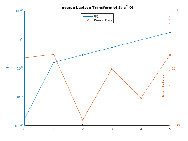
Example
This example computes values of the inverse Laplace transform of the function
The exact answer is
The program first calls
nag_sum_invlaplace_weeks (c06lb) to compute the coefficients of the Laguerre expansion, and then calls
nag_sum_invlaplace_weeks_eval (c06lc) to evaluate the expansion at
,
,
,
,
,
.
Open in the MATLAB editor:
c06lb_example
function c06lb_example
fprintf('c06lb example results\n\n');
sigma0 = 3;
epstol = 1e-5;
b = 0;
sigma = 0;
n = 5;
earray = zeros(1, n+1);
jarray = zeros(1, n+1);
farray = zeros(1, n+1);
parray = zeros(1, n+1);
[sigmaOut, bOut, m, acoef, errvec, ifail] = ...
c06lb(@f, sigma0, sigma, b, epstol);
if ifail ~= 0
error('Warning: c06lb returned with ifail = %1d ',ifail);
end
disp(['No. of coefficients returned by c06lb = ',num2str(m)]);
disp(' ');
disp(' Computed Exact Pseudo');
disp('t f(t) f(t) error');
for j = 0:5
t = double(j);
[finv, ifail] = c06lc(t, sigmaOut, bOut, acoef, errvec, 'm', m);
if ifail ~= 0
error('Warning: c06lc returned with ifail = %1d ',ifail);
end
exact = sinh(3.0*t);
pserr = abs(finv-exact)/exp(sigmaOut*t);
fprintf('%d %10.4d %11.4d %8.4d\n', t, finv, exact, pserr);
jarray(j+1) = t;
farray(j+1) = finv;
parray(j+1) = pserr;
end
fig1 = figure;
display_plot(jarray, farray, parray)
function [f] = f(s)
f=3.0/(s^2-9.0);
if isreal(f)
f=complex(f);
end
function plot(jarray, farray, parray)
[haxes, hline1, hline2] = plotyy(jarray, farray, jarray, parray,...
'semilogy','semilogy');
set(haxes(1), 'YLim', [1.0e-10 1.0e10]);
set(haxes(1), 'YMinorTick', 'on');
set(haxes(1), 'YTick', [1.0e-10 1.0e-5 1.0 1.0e5 1.0e10]);
set(haxes(2), 'YLim', [1.0e-10 1.0e-8]);
set(haxes(2), 'YMinorTick', 'on');
set(haxes(2), 'YTick', [1e-10 1e-9 1e-8]);
for iaxis = 1:2
set(haxes(iaxis), 'XLim', [0 5]);
set(haxes(iaxis), 'XTick', [0 1 2 3 4 5]);
end
set(gca, 'box', 'off');
title('Inverse Laplace Transform of 3/(s^2-9)');
xlabel('t');
ylabel(haxes(1),'f(t)');
ylabel(haxes(2),'Pseudo Error');
legend('f(t)','Pseudo Error','location','North')
set(hline1, 'Linewidth', 0.5, 'Marker', '+', 'LineStyle', '-');
set(hline2, 'Linewidth', 0.5, 'Marker', 'x', 'LineStyle', '-');
function display_plot(jarray, farray, parray)
[haxes, hline1, hline2] = plotyy(jarray, farray, jarray, parray,...
'semilogy','semilogy');
set(haxes(1), 'YLim', [1.0e-10 1.0e10]);
set(haxes(1), 'YMinorTick', 'on');
set(haxes(1), 'YTick', [1.0e-10 1.0e-5 1.0 1.0e5 1.0e10]);
set(haxes(2), 'YLim', [1.0e-10 1.0e-8]);
set(haxes(2), 'YMinorTick', 'on');
set(haxes(2), 'YTick', [1e-10 1e-9 1e-8]);
for iaxis = 1:2
set(haxes(iaxis), 'XLim', [0 5]);
set(haxes(iaxis), 'XTick', [0 1 2 3 4 5]);
end
set(gca, 'box', 'off');
title('Inverse Laplace Transform of 3/(s^2-9)');
xlabel('t');
ylabel(haxes(1),'f(t)');
yh=ylabel(haxes(2),'Pseudo Error');
set(yh, 'position',[4.7,5e-10]);
legend('f(t)','Pseudo Error','location','North')
set(hline1, 'Linewidth', 0.5, 'Marker', '+', 'LineStyle', '-');
set(hline2, 'Linewidth', 0.5, 'Marker', 'x', 'LineStyle', '-');
c06lb example results

No. of coefficients returned by c06lb = 64

      Computed       Exact         Pseudo
t       f(t)          f(t)          error
0   1.5129e-09          0000     1.5129e-09
1   1.0018e+01    1.0018e+01     1.7394e-09
2   2.0171e+02    2.0171e+02     1.2471e-10
3   4.0515e+03    4.0515e+03     9.7722e-10
4   8.1377e+04    8.1377e+04     3.0221e-10
5   1.6345e+06    1.6345e+06     1.6991e-09
PDF version (NAG web site
, 64-bit version, 64-bit version)
© The Numerical Algorithms Group Ltd, Oxford, UK. 2009–2015