hide long namesshow long names
hide short namesshow short names
Integer type:  int32  int64  nag_int  show int32  show int32  show int64  show int64  show nag_int  show nag_int

PDF version (NAG web site, 64-bit version, 64-bit version)
Chapter Contents
Chapter Introduction
NAG Toolbox

NAG Toolbox: nag_tsa_cp_binary_user (g13ne)

 Contents

    1  Purpose
    2  Syntax
    7  Accuracy
    9  Example

Purpose

nag_tsa_cp_binary_user (g13ne) detects change points in a univariate time series, that is, the time points at which some feature of the data, for example the mean, changes. Change points are detected using binary segmentation for a user-supplied cost function.

Syntax

[tau, user, ifail] = g13ne(n, beta, chgpfn, 'minss', minss, 'mdepth', mdepth, 'user', user)
[tau, user, ifail] = nag_tsa_cp_binary_user(n, beta, chgpfn, 'minss', minss, 'mdepth', mdepth, 'user', user)

Description

Let y1:n=yj:j=1,2,,n denote a series of data and τ=τi:i=1,2,,m denote a set of m ordered (strictly monotonic increasing) indices known as change points with 1τin and τm=n. For ease of notation we also define τ0=0. The m change points, τ, split the data into m segments, with the ith segment being of length ni and containing yτi-1+1:τi.
Given a cost function, Cyτi-1+1:τi, nag_tsa_cp_binary_user (g13ne) gives an approximate solution to
minimize m,τ i=1 m Cyτi-1+1:τi + β  
where β is a penalty term used to control the number of change points. The solution is obtained in an iterative manner as follows:
1. Set u=1, w=n and k=0
2. Set k=k+1. If k>K, where K is a user-supplied control parameter, then terminate the process for this segment.
3. Find v that minimizes
Cyu:v + Cyv+1:w  
4. Test
Cyu:v + Cyv+1:w + β < Cyu:w (1)
5. If inequality (1) is false then the process is terminated for this segment.
6. If inequality (1) is true, then v is added to the set of change points, and the segment is split into two subsegments, yu:v and yv+1:w. The whole process is repeated from step 2 independently on each subsegment, with the relevant changes to the definition of u and w (i.e., w is set to v when processing the left hand subsegment and u is set to v+1 when processing the right hand subsegment.
The change points are ordered to give τ.

References

Chen J and Gupta A K (2010) Parametric Statistical Change Point Analysis With Applications to Genetics Medicine and Finance Second Edition Birkhäuser

Parameters

Compulsory Input Parameters

1:     n int64int32nag_int scalar
n, the length of the time series.
Constraint: n2.
2:     beta – double scalar
β, the penalty term.
There are a number of standard ways of setting β, including:
SIC or BIC
β=p×logn.
AIC
β=2p.
Hannan-Quinn
β=2p×loglogn.
where p is the number of parameters being treated as estimated in each segment. The value of p will depend on the cost function being used.
If no penalty is required then set β=0. Generally, the smaller the value of β the larger the number of suggested change points.
3:     chgpfn – function handle or string containing name of m-file
chgpfn must calculate a proposed change point, and the associated costs, within a specified segment.
[v, cost, user, info] = chgpfn(side, u, w, minss, user, info)

Input Parameters

1:     side int64int32nag_int scalar
Flag indicating what chgpfn must calculate and at which point of the Binary Segmentation it has been called.
side=-1
only Cyu:w need be calculated and returned in cost1, neither v nor the other elements of cost need be set. In this case, u=1 and w=n.
side=0
all elements of cost and v must be set. In this case, u=1 and w=n.
side=1
the segment, yu:w, is a left hand side subsegment from a previous iteration of the Binary Segmentation algorithm. All elements of cost and v must be set.
side=2
the segment, yu:w, is a right hand side subsegment from a previous iteration of the Binary Segmentation algorithm. All elements of cost and v must be set.
The distinction between side=1 and 2 may allow for chgpfn to be implemented in a more efficient manner. See section Example for one such example.
The first call to chgpfn will always have side=-1 and the second call will always have side=0. All subsequent calls will be made with side=1 or 2.
2:     u int64int32nag_int scalar
u, the start of the segment of interest.
3:     w int64int32nag_int scalar
w, the end of the segment of interest.
4:     minss int64int32nag_int scalar
The minimum distance between two change points, as passed to nag_tsa_cp_binary_user (g13ne).
5:     user – Any MATLAB object
chgpfn is called from nag_tsa_cp_binary_user (g13ne) with the object supplied to nag_tsa_cp_binary_user (g13ne).
6:     info int64int32nag_int scalar
info=0.

Output Parameters

1:     v int64int32nag_int scalar
If side=-1 then v need not be set.
if side-1 then v, the proposed change point. That is, the value which minimizes
minimize v Cyu:v + Cyv+1:w  
for v=u+minss-1 to w-minss.
2:     cost3 – double array
Costs associated with the proposed change point, v.
If side=-1 then cost1=Cyu:w and the remaining two elements of cost need not be set.
If side-1 then
  • cost1= Cyu:v + Cyv+1:w .
  • cost2= Cyu:v .
  • cost3= Cyv+1:w .
3:     user – Any MATLAB object
4:     info int64int32nag_int scalar
In most circumstances info should remain unchanged.
If info is set to a strictly positive value then nag_tsa_cp_binary_user (g13ne) terminates with ifail=51.
If info is set to a strictly negative value the current segment is skipped (i.e., no change points are considered in this segment) and nag_tsa_cp_binary_user (g13ne) continues as normal. If info was set to a strictly negative value at any point and no other errors occur then nag_tsa_cp_binary_user (g13ne) will terminate with ifail=52.

Optional Input Parameters

1:     minss int64int32nag_int scalar
Default: 2
The minimum distance between two change points, that is τi-τi-1minss.
Constraint: minss2.
2:     mdepth int64int32nag_int scalar
Default: 0
K, the maximum depth for the iterative process, which in turn puts an upper limit on the number of change points with m2K.
If K0 then no limit is put on the depth of the iterative process and no upper limit is put on the number of change points.
3:     user – Any MATLAB object
user is not used by nag_tsa_cp_binary_user (g13ne), but is passed to chgpfn. Note that for large objects it may be more efficient to use a global variable which is accessible from the m-files than to use user.

Output Parameters

1:     tauntau int64int32nag_int array
The dimension of the array tau will be ntau
The location of the change points. The ith segment is defined by yτi-1+1 to yτi, where τ0=0 and τi=taui,1im.
2:     user – Any MATLAB object
3:     ifail int64int32nag_int scalar
ifail=0 unless the function detects an error (see Error Indicators and Warnings).

Error Indicators and Warnings

Errors or warnings detected by the function:

Cases prefixed with W are classified as warnings and do not generate an error of type NAG:error_n. See nag_issue_warnings.

   ifail=11
Constraint: n2.
   ifail=31
Constraint: minss2.
   ifail=51
User requested termination by setting .
W  ifail=52
User requested a segment to be skipped by setting .
   ifail=-99
An unexpected error has been triggered by this routine. Please contact NAG.
   ifail=-399
Your licence key may have expired or may not have been installed correctly.
   ifail=-999
Dynamic memory allocation failed.

Accuracy

Not applicable.

Further Comments

nag_tsa_cp_binary (g13nd) performs the same calculations for a cost function selected from a provided set of cost functions. If the required cost function belongs to this provided set then nag_tsa_cp_binary (g13nd) can be used without the need to provide a cost function routine.

Example

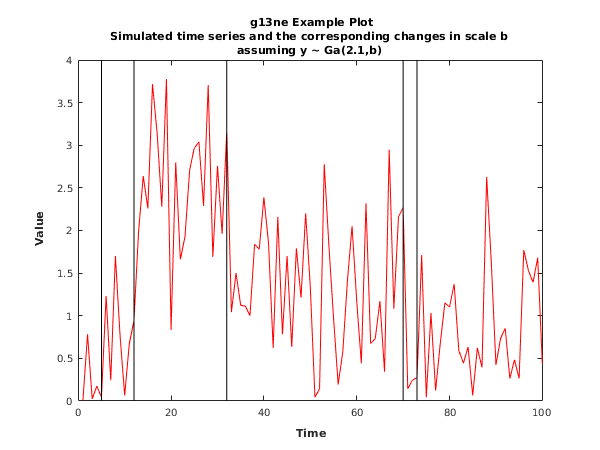
This example identifies changes in the scale parameter, under the assumption that the data has a gamma distribution, for a simulated dataset with 100 observations. A penalty, β of 3.6 is used and the minimum segment size is set to 3. The shape parameter is fixed at 2.1 across the whole input series.
The cost function used is
Cyτi-1+1:τi = 2 a ni logSi - log a ni  
where a is a shape parameter that is fixed for all segments and ni=τi-τi-1+1.
function g13ne_example


fprintf('g13ne example results\n\n');

% Input series
y = [ 0.00; 0.78; 0.02; 0.17; 0.04; 1.23; 0.24; 1.70; 0.77; 0.06;
      0.67; 0.94; 1.99; 2.64; 2.26; 3.72; 3.14; 2.28; 3.78; 0.83;
      2.80; 1.66; 1.93; 2.71; 2.97; 3.04; 2.29; 3.71; 1.69; 2.76;
      1.96; 3.17; 1.04; 1.50; 1.12; 1.11; 1.00; 1.84; 1.78; 2.39;
      1.85; 0.62; 2.16; 0.78; 1.70; 0.63; 1.79; 1.21; 2.20; 1.34;
      0.04; 0.14; 2.78; 1.83; 0.98; 0.19; 0.57; 1.41; 2.05; 1.17;
      0.44; 2.32; 0.67; 0.73; 1.17; 0.34; 2.95; 1.08; 2.16; 2.27;
      0.14; 0.24; 0.27; 1.71; 0.04; 1.03; 0.12; 0.67; 1.15; 1.10;
      1.37; 0.59; 0.44; 0.63; 0.06; 0.62; 0.39; 2.63; 1.63; 0.42;
      0.73; 0.85; 0.26; 0.48; 0.26; 1.77; 1.53; 1.39; 1.68; 0.43];

% Shape parameter used in the cost function
a = 2.1;

% Length of the input series
n = int64(numel(y));

% Need some persisteny workspace in the user function
work = zeros(2*n,1);

% The input series, workspace and shape parameter
% constitute the information that needs to be passed to the
% costfun, so pack them together into a cell array which will
% get passed through the NAG function
user = {y; a; work};

% Penalty term
beta = 3.4;

% Drop small regions
minss = int64(3);

[tau] = g13ne(n,beta,@chgpfn,'minss',minss,'user',user);

% Print the results
fprintf('  -- Change Points --\n');
fprintf('  Number     Position\n');
fprintf(' =====================\n');
for i = 1:numel(tau)
  fprintf(' %4d       %6d\n', i, tau(i));
end

% Plot the results
fig1 = figure;

% Plot the original series
plot(y,'Color','red');

% Mark the change points, drop the last one as it is always
% at the end of the series
xpos = transpose(double(tau(1:end-1))*ones(1,2));
ypos = diag(ylim)*ones(2,numel(tau)-1);
line(xpos,ypos,'Color','black');

% Add labels and titles
title({'{\bf g13ne Example Plot}',
       'Simulated time series and the corresponding changes in scale b',
       'assuming y ~ Ga(2.1,b)'});
xlabel('{\bf Time}');
ylabel('{\bf Value}');


function [v,cost,user,info] = chgpfn(side,u,w,minss,user,info)
  % Function to calculate a proposed change point and associated cost
  % The cost is based on the likelihood of the gamma distribution
  y = user{1};
  a = user{2};
  work = user{3};

  % Calculate the first and last positions for potential change
  % points, conditional on the fact that each sub-segment must be
  % at least minss wide
  floc = u + minss - 1;
  lloc = w - minss;
  
  % In order to calculate the cost of having a change point at i, we
  % need to calculate C(y(floc:i)) and C(y(i+1:lloc)), where C(.) is
  % the cost function (based on the gamma distribution in this example).
  % Rather than calculate these values at each call to chgpfn we store
  % the values in work for later use

  % If side = 1 (i.e. we are working with a left hand sub-segment),
  % we already have C(y(floc:i)) for this value of floc, so only need
  % to calculate C(y(i+1:lloc)), similarly when side = 2 we only need
  % to calculate C(y(floc:i))
  % When side = -1, we need the cost of the full segment, which we do
  % in a forwards manner (calculating C(y(floc:i)) in the process), so
  % when side = 0 we only need to calculate C(y(i:1:lloc))

  % Get the intermediate costs
  ys = 0;
  dn = 0;
  if (side==0 | side==1)
    % work(2*i) = C(y(i+1:w))
    for i = w:-1:floc + 1
      dn = dn + 1;
      tmp = dn*a;
      ys = ys + y(i);
      work(2*i-2) = 2.0*tmp*(log(ys)-log(tmp));
    end

    % make sure we return the updated values of work
    user = {y; a; work};

  else
    % work(2*i-1) = C(y(u:i))
    if (side==-1)
      li = w;
    else
      li = lloc;
    end
    for i = u:li
      dn = dn + 1;
      tmp = dn*a;
      ys = ys + y(i);
      work(2*i-1) = 2.0*tmp*(log(ys)-log(tmp));
    end

    % make sure we return the updated values of work
    user = {y; a; work};
  end

  v = int64(0);
  cost = zeros(3,1);
  if (side>=0)
    % Need to find a potential change point
    v = int64(0);
    cost(1) = 0;

    % Loop over all possible change point locations
    for i = floc:lloc
      this_cost = work(2*i-1) + work(2*i);

      if (this_cost<cost(1) | v==0)
        % Update the proposed change point location
        v = int64(i);
        cost(1) = this_cost;
        cost(2) = work(2*i-1);
        cost(3) = work(2*i);
      end
    end

  else
    % Need to calculate the cost for the full segment
    cost(1) = work(2*w-1);

  % No need to populate the rest of COST or V
  end

  % Set info nonzero to terminate execution for any reason
  info = int64(0);
g13ne example results

  -- Change Points --
  Number     Position
 =====================
    1            5
    2           12
    3           32
    4           70
    5           73
    6          100
g13ne_fig1.png
This example plot shows the original data series and the estimated change points.

PDF version (NAG web site, 64-bit version, 64-bit version)
Chapter Contents
Chapter Introduction
NAG Toolbox

© The Numerical Algorithms Group Ltd, Oxford, UK. 2009–2015