nag_rand_field_2d_predef_setup (g05zr) performs the setup required in order to simulate stationary Gaussian random fields in two dimensions, for a preset variogram, using the circulant embedding method. Specifically, the eigenvalues of the extended covariance matrix (or embedding matrix) are calculated, and their square roots output, for use by nag_rand_field_2d_generate (g05zs), which simulates the random field.

Syntax

[lam, xx, yy, m, approx, rho, icount, eig, ifail] = g05zr(ns, xmin, xmax, ymin, ymax, maxm, var, icov2, params, 'norm_p', norm_p, 'np', np, 'pad', pad, 'icorr', icorr)

[lam, xx, yy, m, approx, rho, icount, eig, ifail] = nag_rand_field_2d_predef_setup(ns, xmin, xmax, ymin, ymax, maxm, var, icov2, params, 'norm_p', norm_p, 'np', np, 'pad', pad, 'icorr', icorr)

Description

A two-dimensional random field

Z (x)

ℝ^{2}

is a function which is random at every point

x \in ℝ^{2}

, so

Z (x)

is a random variable for each

x

. The random field has a mean function

μ (x) = 𝔼 [Z (x)]

and a symmetric positive semidefinite covariance function

C (x, y) = 𝔼 [(Z (x) - μ (x)) (Z (y) - μ (y))]

Z (x)

is a Gaussian random field if for any choice of

n \in ℕ

and

x_{1}, \dots, x_{n} \in ℝ^{2}

, the random vector

{[Z (x_{1}), \dots, Z (x_{n})]}^{T}

follows a multivariate Normal distribution, which would have a mean vector

\tilde{μ}

with entries

{\tilde{μ}}_{i} = μ (x_{i})

and a covariance matrix

\tilde{C}

with entries

{\tilde{C}}_{i j} = C (x_{i}, x_{j})

. A Gaussian random field

Z (x)

is stationary if

μ (x)

is constant for all

x \in ℝ^{2}

and

C (x, y) = C (x + a, y + a)

for all

x, y, a \in ℝ^{2}

and hence we can express the covariance function

C (x, y)

as a function

γ

of one variable:

C (x, y) = γ (x - y)

γ

is known as a variogram (or more correctly, a semivariogram) and includes the multiplicative factor

σ^{2}

representing the variance such that

γ (0) = σ^{2}

The functions nag_rand_field_2d_predef_setup (g05zr) and nag_rand_field_2d_generate (g05zs) are used to simulate a two-dimensional stationary Gaussian random field, with mean function zero and variogram

γ (x)

, over a domain

[x_{\min}, x_{\max}] \times [y_{\min}, y_{\max}]

, using an equally spaced set of

N_{1} \times N_{2}

points;

N_{1}

points in the

x

-direction and

N_{2}

points in the

y

-direction. The problem reduces to sampling a Gaussian random vector

X

of size

N_{1} \times N_{2}

, with mean vector zero and a symmetric covariance matrix

A

, which is an

N_{2}

N_{2}

block Toeplitz matrix with Toeplitz blocks of size

N_{1}

N_{1}

. Since

A

is in general expensive to factorize, a technique known as the circulant embedding method is used.

A

is embedded into a larger, symmetric matrix

B

, which is an

M_{2}

M_{2}

block circulant matrix with circulant blocks of size

M_{1}

M_{1}

, where

M_{1} \geq 2 (N_{1} - 1)

and

M_{2} \geq 2 (N_{2} - 1)

B

can now be factorized as

B = W Λ W^{*} = R^{*} R

, where

W

is the two-dimensional Fourier matrix (

W^{*}

is the complex conjugate of

W

Λ

is the diagonal matrix containing the eigenvalues of

B

and

R = Λ^{\frac{1}{2}} W^{*}

B

is known as the embedding matrix. The eigenvalues can be calculated by performing a discrete Fourier transform of the first row (or column) of

B

and multiplying by

M_{1} \times M_{2}

, and so only the first row (or column) of

B

is needed – the whole matrix does not need to be formed.

As long as all of the values of

Λ

are non-negative (i.e.,

B

is positive semidefinite),

B

is a covariance matrix for a random vector

Y

which has

M_{2}

blocks of size

M_{1}

. Two samples of

Y

can now be simulated from the real and imaginary parts of

R^{*} (U + i V)

, where

U

and

V

have elements from the standard Normal distribution. Since

R^{*} (U + i V) = W Λ^{\frac{1}{2}} (U + i V)

, this calculation can be done using a discrete Fourier transform of the vector

Λ^{\frac{1}{2}} (U + i V)

. Two samples of the random vector

X

can now be recovered by taking the first

N_{1}

elements of the first

N_{2}

blocks of each sample of

Y

– because the original covariance matrix

A

is embedded in

B

X

will have the correct distribution.

B

is not positive semidefinite, larger embedding matrices

B

can be tried; however if the size of the matrix would have to be larger than maxm, an approximation procedure is used. We write

Λ = Λ_{+} + Λ_{-}

, where

Λ_{+}

and

Λ_{-}

contain the non-negative and negative eigenvalues of

B

respectively. Then

B

is replaced by

ρ B_{+}

where

B_{+} = W Λ_{+} W^{*}

and

ρ \in (0, 1]

is a scaling factor. The error

ε

in approximating the distribution of the random field is given by

ε = \sqrt{\frac{{(1 - ρ)}^{2} trace Λ + ρ^{2} trace Λ_{-}}{M}} .

Three choices for

ρ

are available, and are determined by the input argument icorr:

setting $icorr = 0$ sets
$ρ = \frac{trace Λ}{trace Λ_{+}},$
setting $icorr = 1$ sets
$ρ = \sqrt{\frac{trace Λ}{trace Λ_{+}}},$
setting $icorr = 2$ sets $ρ = 1$ .

nag_rand_field_2d_predef_setup (g05zr) finds a suitable positive semidefinite embedding matrix

B

and outputs its sizes in the vector m and the square roots of its eigenvalues in lam. If approximation is used, information regarding the accuracy of the approximation is output. Note that only the first row (or column) of

B

is actually formed and stored.

References

Dietrich C R and Newsam G N (1997) Fast and exact simulation of stationary Gaussian processes through circulant embedding of the covariance matrix SIAM J. Sci. Comput. 18 1088–1107

Schlather M (1999) Introduction to positive definite functions and to unconditional simulation of random fields Technical Report ST 99–10 Lancaster University

Wood A T A and Chan G (1997) Algorithm AS 312: An Algorithm for Simulating Stationary Gaussian Random Fields Journal of the Royal Statistical Society, Series C (Applied Statistics) (Volume 46) 1 171–181

Parameters

Compulsory Input Parameters

1: $ns (2)$ – int64int32nag_int array

The number of sample points to use in each direction, with

ns (1)

sample points in the

x

-direction,

N_{1}

and

ns (2)

sample points in the

y

-direction,

N_{2}

. The total number of sample points on the grid is therefore

ns (1) \times ns (2)

Constraints:

$ns (1) \geq 1$ ;
$ns (2) \geq 1$ .

2: $xmin$ – double scalar

The lower bound for the

x

-coordinate, for the region in which the random field is to be simulated.

Constraint:

xmin < xmax

3: $xmax$ – double scalar

The upper bound for the

x

-coordinate, for the region in which the random field is to be simulated.

Constraint:

xmin < xmax

4: $ymin$ – double scalar

The lower bound for the

y

-coordinate, for the region in which the random field is to be simulated.

Constraint:

ymin < ymax

5: $ymax$ – double scalar

The upper bound for the

y

-coordinate, for the region in which the random field is to be simulated.

Constraint:

ymin < ymax

6: $maxm (2)$ – int64int32nag_int array

Determines the maximum size of the circulant matrix to use – a maximum of

maxm (1)

elements in the

x

-direction, and a maximum of

maxm (2)

elements in the

y

-direction. The maximum size of the circulant matrix is thus

maxm (1)

\times

maxm (2)

Constraint:

maxm (i) \geq 2^{k}

, where

k

is the smallest integer satisfying

2^{k} \geq 2 (ns (i) - 1)

, for

i = 1, 2

7: $var$ – double scalar

The multiplicative factor

σ^{2}

of the variogram

γ (x)

Constraint:

var \geq 0.0

8: $icov2$ – int64int32nag_int scalar

Determines which of the preset variograms to use. The choices are given below. Note that

x^{'} = ‖\frac{x}{ℓ_{1}}, \frac{y}{ℓ_{2}}‖

, where

ℓ_{1}

and

ℓ_{2}

are correlation lengths in the

x

and

y

directions respectively and are parameters for most of the variograms, and

σ^{2}

is the variance specified by var.

$icov2 = 1$

Symmetric stable variogram

γ (x) = σ^{2} \exp (- {(x^{'})}^{ν}),

where

$ℓ_{1} = params (1)$ , $ℓ_{1} > 0$ ,
$ℓ_{2} = params (2)$ , $ℓ_{2} > 0$ ,
$ν = params (3)$ , $0 < ν \leq 2$ .

$icov2 = 2$

Cauchy variogram

γ (x) = σ^{2} {(1 + {(x^{'})}^{2})}^{- ν},

where

$ℓ_{1} = params (1)$ , $ℓ_{1} > 0$ ,
$ℓ_{2} = params (2)$ , $ℓ_{2} > 0$ ,
$ν = params (3)$ , $ν > 0$ .

$icov2 = 3$

Differential variogram with compact support

γ (x) = \{\begin{matrix} σ^{2} (1 + 8 x^{'} + 25 {(x^{'})}^{2} + 32 {(x^{'})}^{3}) {(1 - x^{'})}^{8}, & x^{'} < 1, \\ 0, & x^{'} \geq 1, \end{matrix}

where

$ℓ_{1} = params (1)$ , $ℓ_{1} > 0$ ,
$ℓ_{2} = params (2)$ , $ℓ_{2} > 0$ .

$icov2 = 4$

Exponential variogram

γ (x) = σ^{2} \exp (- x^{'}),

where

$ℓ_{1} = params (1)$ , $ℓ_{1} > 0$ ,
$ℓ_{2} = params (2)$ , $ℓ_{2} > 0$ .

$icov2 = 5$

Gaussian variogram

γ (x) = σ^{2} \exp ({- (x^{'})}^{2}),

where

$ℓ_{1} = params (1)$ , $ℓ_{1} > 0$ ,
$ℓ_{2} = params (2)$ , $ℓ_{2} > 0$ .

$icov2 = 6$

Nugget variogram

γ (x) = \{\begin{matrix} σ^{2}, & x = 0, \\ 0, & x \neq 0 . \end{matrix}

No parameters need be set for this value of icov2.

$icov2 = 7$

Spherical variogram

γ (x) = \{\begin{matrix} σ^{2} (1 - 1.5 x^{'} + 0.5 {(x^{'})}^{3}), & x^{'} < 1, \\ 0, & x^{'} \geq 1, \end{matrix}

where

$ℓ_{1} = params (1)$ , $ℓ_{1} > 0$ ,
$ℓ_{2} = params (2)$ , $ℓ_{2} > 0$ .

$icov2 = 8$

Bessel variogram

γ (x) = σ^{2} \frac{2^{ν} Γ (ν + 1) J_{ν} (x^{'})}{{(x^{'})}^{ν}},

where

$J_{ν} (\cdot)$ is the Bessel function of the first kind,
$ℓ_{1} = params (1)$ , $ℓ_{1} > 0$ ,
$ℓ_{2} = params (2)$ , $ℓ_{2} > 0$ ,
$ν = params (3)$ , $ν \geq 0$ .

$icov2 = 9$

Hole effect variogram

γ (x) = σ^{2} \frac{\sin (x^{'})}{x^{'}},

where

$ℓ_{1} = params (1)$ , $ℓ_{1} > 0$ ,
$ℓ_{2} = params (2)$ , $ℓ_{2} > 0$ .

$icov2 = 10$

Whittle-Matérn variogram

γ (x) = σ^{2} \frac{2^{1 - ν} {(x^{'})}^{ν} K_{ν} (x^{'})}{Γ (ν)},

where

$K_{ν} (\cdot)$ is the modified Bessel function of the second kind,
$ℓ_{1} = params (1)$ , $ℓ_{1} > 0$ ,
$ℓ_{2} = params (2)$ , $ℓ_{2} > 0$ ,
$ν = params (3)$ , $ν > 0$ .

$icov2 = 11$

Continuously parameterised variogram with compact support

γ (x) = \{\begin{matrix} σ^{2} \frac{2^{1 - ν} {(x^{'})}^{ν} K_{ν} (x^{'})}{Γ (ν)} (1 + 8 x^{''} + 25 {(x^{''})}^{2} + 32 {(x^{''})}^{3}) {(1 - x^{''})}^{8}, & x^{''} < 1, \\ 0, & x^{''} \geq 1, \end{matrix}

where

$x^{′′} = ‖\frac{x^{'}}{ℓ_{1} s_{1}}, \frac{y^{'}}{ℓ_{2} s_{2}}‖$ ,
$K_{ν} (\cdot)$ is the modified Bessel function of the second kind,
$ℓ_{1} = params (1)$ , $ℓ_{1} > 0$ ,
$ℓ_{2} = params (2)$ , $ℓ_{2} > 0$ ,
$s_{1} = params (3)$ , $s_{1} > 0$ ,
$s_{2} = params (4)$ , $s_{2} > 0$ ,
$ν = params (5)$ , $ν > 0$ .

$icov2 = 12$

Generalized hyperbolic distribution variogram

γ (x) = σ^{2} \frac{{(δ^{2} + {(x^{'})}^{2})}^{\frac{λ}{2}}}{δ^{λ} K_{λ} (κ δ)} K_{λ} (κ {(δ^{2} + {(x^{'})}^{2})}^{\frac{1}{2}}),

where

$K_{λ} (\cdot)$ is the modified Bessel function of the second kind,
$ℓ_{1} = params (1)$ , $ℓ_{1} > 0$ ,
$ℓ_{2} = params (2)$ , $ℓ_{2} > 0$ ,
$λ = params (3)$ , no constraint on $λ$ ,
$δ = params (4)$ , $δ > 0$ ,
$κ = params (5)$ , $κ > 0$ .

Constraint:

icov2 = 1

2

3

4

5

6

7

8

9

10

11

12

9: $params (np)$ – double array

The parameters for the variogram as detailed in the description of icov2.

Constraint: see icov2 for a description of the individual parameter constraints.

Optional Input Parameters

1: $norm_p$ – int64int32nag_int scalar

Default:

norm_p = 2

Determines which norm to use when calculating the variogram.

$norm_p = 1$: The 1-norm is used, i.e., $‖x, y‖ = |x| + |y|$ .
$norm_p = 2$: The 2-norm (Euclidean norm) is used, i.e., $‖x, y‖ = \sqrt{x^{2} + y^{2}}$ .

Constraint:

norm_p = 1

2

2: $np$ – int64int32nag_int scalar

Default: the dimension of the array params.

The number of parameters to be set. Different covariance functions need a different number of parameters.

$icov2 = 6$: np must be set to $0$ .
$icov2 = 3$ , $4$ , $5$ , $7$ or $9$: np must be set to $2$ .
$icov2 = 1$ , $2$ , $8$ or $10$: np must be set to $3$ .
$icov2 = 11$ or $12$: np must be set to $5$ .

3: $pad$ – int64int32nag_int scalar

Default:

pad = 1

Determines whether the embedding matrix is padded with zeros, or padded with values of the variogram. The choice of padding may affect how big the embedding matrix must be in order to be positive semidefinite.

$pad = 0$: The embedding matrix is padded with zeros.
$pad = 1$: The embedding matrix is padded with values of the variogram.

Constraint:

pad = 0

1

4: $icorr$ – int64int32nag_int scalar

Default:

icorr = 0

Determines which approximation to implement if required, as described in Description.

Constraint:

icorr = 0

1

2

Output Parameters

1: $lam (maxm (1) \times maxm (2))$ – double array

Contains the square roots of the eigenvalues of the embedding matrix.

2: $xx (ns (1))$ – double array

The points of the

x

-coordinates at which values of the random field will be output.

3: $yy (ns (2))$ – double array

The points of the

y

-coordinates at which values of the random field will be output.

4: $m (2)$ – int64int32nag_int array

m (1)

contains

M_{1}

, the size of the circulant blocks and

m (2)

contains

M_{2}

, the number of blocks, resulting in a final square matrix of size

M_{1} \times M_{2}

5: $approx$ – int64int32nag_int scalar

Indicates whether approximation was used.

$approx = 0$: No approximation was used.
$approx = 1$: Approximation was used.

6: $rho$ – double scalar

Indicates the scaling of the covariance matrix.

rho = 1.0

unless approximation was used with

icorr = 0

1

7: $icount$ – int64int32nag_int scalar

Indicates the number of negative eigenvalues in the embedding matrix which have had to be set to zero.

8: $eig (3)$ – double array

Indicates information about the negative eigenvalues in the embedding matrix which have had to be set to zero.

eig (1)

contains the smallest eigenvalue,

eig (2)

contains the sum of the squares of the negative eigenvalues, and

eig (3)

contains the sum of the absolute values of the negative eigenvalues.

9: $ifail$ – int64int32nag_int scalar

ifail = 0

unless the function detects an error (see Error Indicators and Warnings).

Error Indicators and Warnings

Errors or warnings detected by the function:

$ifail = 1$: Constraint: $ns (1) \geq 1$ , $ns (2) \geq 1$ .

$ifail = 2$: Constraint: $xmin < xmax$ .

$ifail = 4$: Constraint: $ymin < ymax$ .

$ifail = 6$: Constraint: the minimum calculated value for maxm are $[_,_]$ .
Where the minima of $maxm (i)$ is given by $2^{k}$ , where $k$ is the smallest integer satisfying $2^{k} \geq 2 (ns (i) - 1)$ , for $i = 1, 2$ .

$ifail = 7$: Constraint: $var \geq 0.0$ .

$ifail = 8$: Constraint: $icov2 \geq 1$ and $icov2 \leq 12$ .

$ifail = 9$: Constraint: $norm_p = 1$ or $2$ .

$ifail = 10$: Constraint: for $icov2 =_$ , $np =_$ .

$ifail = 11$: Constraint: dependent on icov2, see documentation.

$ifail = 12$: Constraint: $pad = 0$ or $1$ .

$ifail = 13$: Constraint: $icorr = 0$ , $1$ or $2$ .

$ifail = - 99$: An unexpected error has been triggered by this routine. Please contact NAG.

$ifail = - 399$: Your licence key may have expired or may not have been installed correctly.

$ifail = - 999$: Dynamic memory allocation failed.

Accuracy

If on exit

approx = 1

, see the comments in Description regarding the quality of approximation; increase the values in maxm to attempt to avoid approximation.

Further Comments

None.

Example

This example calls nag_rand_field_2d_predef_setup (g05zr) to calculate the eigenvalues of the embedding matrix for

25

sample points on a

5

5

grid of a two-dimensional random field characterized by the symmetric stable variogram (

icov2 = 1

Open in the MATLAB editor: g05zr_example

function g05zr_example


fprintf('g05zr example results\n\n');

% Use symmetric stable variogram
icov2 = int64(1);
params = [0.1; 0.15; 1.2];

% Random Field variance
var = 0.5;
% Domain endpoints
xmin = -1;
xmax =  1;
ymin = -0.5;
ymax =  0.5;
% Number of sample points in x and y
ns = [int64(5), 5];
% Maximum dimensions of circulant matrix
maxm = [int64(64), 64];
% Scaling factor, rhoo = 1.
icorr = int64(2);

% Get square roots of the eigenvalues of the embedding matrix
[lam, xx, yy, m, approx, rho, icount, eig, ifail] = ...
  g05zr( ...
         ns, xmin, xmax, ymin, ymax, maxm, var, ...
         icov2, params, 'icorr', icorr);

fprintf('Size of embedding matrix = %d\n\n', m(1)*m(2));

% Display approximation information if approximation used
if approx == 1
  fprintf('Approximation required\n\n');
  fprintf('rho = %10.5f\n', rho);
  fprintf('eig = %10.5f%10.5f%10.5f\n', eig(1:3));
  fprintf('icount = %d\n', icount);
else
  fprintf('Approximation not required\n\n');
end

% Display square roots of the eigenvalues of the embedding matrix
fprintf('Square roots of eigenvalues of embedding matrix:\n');
mlam = reshape(lam(1:m(1)*m(2)), m(1), m(2));
for i = 1:m(1)
  fprintf('%8.4f',mlam(i,:));
  fprintf('\n');
end

g05zr_plot;



function g05zr_plot

  icov2 = int64(4);
  params = [0.1; 0.1];
  var = 1;
  % Domain endpoints
  xmin = 0;
  xmax = 1;
  ymin = 0;
  ymax = 1;
  % Number of sample points in x and y
  ns = [int64(100), 100];
  % Maximum dimensions of circulant matrix
  maxm = [int64(4096), 4096];
  icorr = int64(0);

  % Get square roots of the eigenvalues of the embedding matrix
  [lam, xx, yy, m, approx, rho, icount, eig, ifail] = ...
  g05zr( ...
         ns, xmin, xmax, ymin, ymax, maxm, var, ...
         icov2, params);

  % Initialize state array
  genid = int64(1);
  subid = int64(1);
  seed  = [int64(14965)];
  [state, ifail] = g05kf( ...
                          genid, subid, seed);

  % Compute 2 random field realisations
  s = int64(2);
  [state, z, ifail] = g05zs( ...
                             ns, s, m, lam, rho, state);

  fig1 = figure;
  zz = reshape(z(:,1),[100,100]);
  contourf(xx,yy,zz);
  axis equal;
  title({'First realization of Random Field', ...
	 'exponential variogram, corr. length = 0.1'});

  fig2 = figure;
  zz = reshape(z(:,2),[100,100]);
  contourf(xx,yy,zz);
  axis equal;
  title({'Second realization of Random Field', ...
	 'exponential variogram, corr. length = 0.1'});

g05zr example results

Size of embedding matrix = 64

Approximation not required

Square roots of eigenvalues of embedding matrix:
  0.8966  0.8234  0.6810  0.5757  0.5391  0.5757  0.6810  0.8234
  0.8940  0.8217  0.6804  0.5756  0.5391  0.5756  0.6804  0.8217
  0.8877  0.8175  0.6792  0.5754  0.5391  0.5754  0.6792  0.8175
  0.8813  0.8133  0.6780  0.5751  0.5390  0.5751  0.6780  0.8133
  0.8787  0.8116  0.6774  0.5750  0.5390  0.5750  0.6774  0.8116
  0.8813  0.8133  0.6780  0.5751  0.5390  0.5751  0.6780  0.8133
  0.8877  0.8175  0.6792  0.5754  0.5391  0.5754  0.6792  0.8175
  0.8940  0.8217  0.6804  0.5756  0.5391  0.5756  0.6804  0.8217

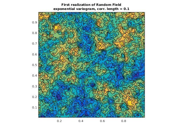
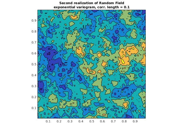
The two plots shown below illustrate the random fields that can be generated by nag_rand_field_2d_generate (g05zs) using the eigenvalues calculated by nag_rand_field_2d_predef_setup (g05zr). These are for two realizations of a two-dimensional random field, based on eigenvalues of the embedding matrix for points on a

100

100

grid. The random field is characterized by the exponential variogram (

icov2 = 4

) with correlation lengths both equal to

0.1

PDF version (NAG web site, 64-bit version, 64-bit version)

Chapter Contents

Chapter Introduction

NAG Toolbox