then an algorithm based directly on the gamma distribution's PDF is used. For values outside this range, the function is calculated via the Poisson distribution's PDF as described in Loader (2000) (see Further Comments).

References

Loader C (2000) Fast and accurate computation of binomial probabilities (not yet published)

Parameters

Compulsory Input Parameters

1: $x$ – double scalar

x

, the value at which the PDF is to be evaluated.

2: $a$ – double scalar

α

, the shape argument of the gamma distribution.

Constraint:

a > 0.0

3: $b$ – double scalar

β

, the scale argument of the gamma distribution.

Constraints:

$b > 0.0$ ;
$\frac{x}{b} < \frac{1}{x02am ()}$ .

Optional Input Parameters

None.

Output Parameters

1: $result$ – double scalar: The result of the function.
2: $ifail$ – int64int32nag_int scalar: $ifail = 0$ unless the function detects an error (see Error Indicators and Warnings).

Error Indicators and Warnings

Errors or warnings detected by the function:

ifail \neq 0

, then nag_stat_pdf_gamma (g01kf) returns

0.0

$ifail = 1$: Constraint: $a > 0.0$ .

$ifail = 2$: Constraint: $b > 0.0$ .

$ifail = 3$: Computation abandoned owing to overflow due to extreme parameter values.

$ifail = - 99$: An unexpected error has been triggered by this routine. Please contact NAG.

$ifail = - 399$: Your licence key may have expired or may not have been installed correctly.

$ifail = - 999$: Dynamic memory allocation failed.

Accuracy

Not applicable.

Further Comments

Due to the lack of a stable link to Loader (2000) paper, we give a brief overview of the method, as applied to the Poisson distribution. The Poisson distribution has a continuous mass function given by,

p (x; λ) = \frac{λ^{x}}{x!} e^{- λ} .

(1)

The usual way of computing this quantity would be to take the logarithm and calculate,

\log (x; λ) = x \log λ - \log (x!) - λ .

For large

x

and

λ

x \log λ

and

\log (x!)

are very large, of the same order of magnitude and when calculated have rounding errors. The subtraction of these two terms can therefore result in a number, many orders of magnitude smaller and hence we lose accuracy due to subtraction errors. For example for

x = 2 \times 10^{6}

and

λ = 2 \times 10^{6}

\log (x!) \approx 2.7 \times 10^{7}

and

\log (p (x; λ)) = - 8.17326744645834

. But calculated with the method shown later we have

\log (p (x; λ)) = - 8.1732674441334492

. The difference between these two results suggests a loss of about 7 significant figures of precision.

Loader introduces an alternative way of expressing (1) based on the saddle point expansion,

\log (p (x; λ)) = \log (p (x; x)) - D (x; λ),

(2)

where

D (x; λ)

, the deviance for the Poisson distribution is given by,

\begin{matrix} D (x; λ) & = & \log (p (x; x)) - \log (p (x; λ)), \\ = & λ D_{0} (\frac{x}{λ}), \end{matrix}

(3)

and

D_{0} (ε) = ε \log ε + 1 - ε .

For

ε

close to

1

D_{0} (ε)

can be evaluated through the series expansion

λ D_{0} (\frac{x}{λ}) = \frac{{(x - λ)}^{2}}{x + λ} + 2 x \sum_{j = 1}^{\infty} \frac{v^{2 j + 1}}{2 j + 1},   where ​ v = \frac{x - λ}{x + λ},

otherwise

D_{0} (ε)

can be evaluated directly. In addition, Loader suggests evaluating

\log (x!)

using the Stirling–De Moivre series,

\log (x!) = \frac{1}{2} \log (2 π x) + x \log (x) - x + δ (x),

(4)

where the error

δ (x)

is given by

δ (x) = \frac{1}{12 x} - \frac{1}{{360 x}^{3}} + \frac{1}{{1260 x}^{5}} + O (x^{- 7}) .

Finally

\log (p (x; λ))

can be evaluated by combining equations (1)–(4) to get,

p (x; λ) = \frac{1}{\sqrt{2 π x}} e^{- δ (x) - λ D_{0} (x / λ)} .

Example

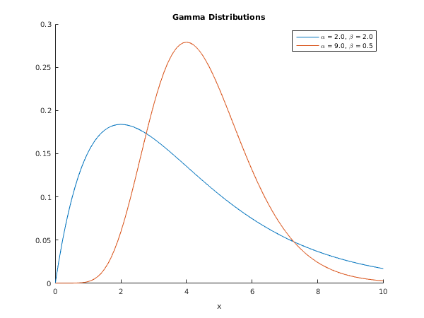
This example prints the value of the gamma distribution PDF at six different points x with differing a and b.

Open in the MATLAB editor: g01kf_example

function g01kf_example


fprintf('g01kf example results\n\n');

x      = [0.1, 3, 6,  4,   9,  16];
a      = [3,  10, 5, 10,   9,   3.5];
b      = [2,  11, 1,  0.1, 0.5, 2.5];
result = x;
fprintf('\n      x            a            b          pdf\n');

for i=1:numel(x)
 [result(i), ifail] = g01kf( ...
			     x(i), a(i), b(i));
end

fprintf('%12.4e %12.4e %12.4e %12.4e\n', [x; a; b; result]);

g01kf_plot;



function g01kf_plot
 
  fig1 = figure;
  hold on;
  a  = [2, 9];
  b  = [2, 0.5];
  x  = [0:0.1:10];
  alpha = '\alpha';
  beta  = '\beta';
  for i=1:2
    for j=1:numel(x)
      [y{i}(j), ifail] = g01kf( ...
				x(j), a(i), b(i));
    end
    plot(x,y{i});
    l{i} = sprintf('%s = %3.1f, %s = %3.1f', alpha, a(i), beta, b(i));
  end
  legend(l);
  xlabel('x');
  title('Gamma Distributions');
  hold off;

g01kf example results


      x            a            b          pdf
  1.0000e-01   3.0000e+00   2.0000e+00   5.9452e-04
  3.0000e+00   1.0000e+01   1.1000e+01   1.5921e-12
  6.0000e+00   5.0000e+00   1.0000e+00   1.3385e-01
  4.0000e+00   1.0000e+01   1.0000e-01   3.0690e-08
  9.0000e+00   9.0000e+00   5.0000e-01   8.3251e-03
  1.6000e+01   3.5000e+00   2.5000e+00   2.0723e-02

PDF version (NAG web site, 64-bit version, 64-bit version)

Chapter Contents

Chapter Introduction

NAG Toolbox