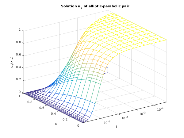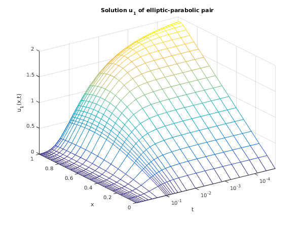
| On entry, | or , |
| or | , |
| or | , |
| or | , |
| or | , or , |
| or | the mesh points , for , are not in strictly increasing order. |
Open in the MATLAB editor: d03pz_example
function d03pz_example


fprintf('d03pz example results\n\n');

%  Solution of an elliptic-parabolic pair of PDEs.
global alpha;

% Set values for problem parameters.
npde = 2;

% Number of points on calculation mesh, and on interpolated mesh.
npts = 20;
intpts = 6;

itype  = int64(1);
neqn   = npde*npts;
lisave = neqn + 24;
nwk    = (10 + 6*npde)*neqn;
lrsave = nwk + (21 + 3*npde)*npde + 7*npts + 54;

% Define some arrays.
rsave  = zeros(lrsave, 1);
u      = zeros(npde, npts);
uinterp = zeros(npde, intpts, itype);
x     = zeros(npts, 1);
isave = zeros(lisave, 1, 'int64');
cwsav = {''; ''; ''; ''; ''; ''; ''; ''; ''; ''};
lwsav = false(100, 1);
iwsav = zeros(505, 1, 'int64');
rwsav = zeros(1100, 1);

% Set up the points on the interpolation grid.
xinterp = [0.0 0.4 0.6 0.8 0.9 1.0];

acc = 1.0e-3;
alpha = 1;

itrace = int64(0);
itask  = int64(1);
% Use cylindrical polar coordinates.
m = int64(1);

% We run through the calculation twice; once to output the interpolated
% results, and once to store the results for plotting.
niter = [5, 28];

% Prepare to store plotting results.
tsav = zeros(niter(2), 1);
usav = zeros(2, niter(2), npts);
isav = 0;

for icalc = 1:2

  % Set spatial mesh points.
  piby2 = pi/2;
  hx = piby2/(npts-1);
  x = sin(0:hx:piby2);

  % Set initial conditions.
  ts   = 0;
  tout = 1e-5;

  % Set the initial values.
  [u] = uinit(x, npts);

  % Start the integration in time.
  ind = int64(0);

  % Counter for saved results.
  isav = 0;

  % Loop over endpoints for the integration.
  % Set itask = 1: normal computation of output values at t = tout.
  for iter = 1:niter(icalc)

    %Set the endpoint.
    if icalc == 1
      tout = 10.0*tout;
    else
      if iter < 10
        tout = 2*tout;
      else
        if iter == 10
          tout = 0.01;
        else
          if iter < 20
            tout = tout + 0.01;
          else
            tout = tout + 0.1;
          end
        end
      end
    end

    % The first time this is called, ind is 0, which (re)starts the
    % integration in time.  On exit, ind is set to 1; using this value
    % on a subsequent call continues the integration.  This means that
    % only tout and ifail should be reset between calls.
    [ts, u, rsave, isave, ind, user, cwsav, lwsav, iwsav, rwsav, ifail] = ...
    d03pc(...
           m, ts, tout, @pdedef, @bndary, u, x, acc, rsave, isave, itask, ...
          itrace, ind, cwsav, lwsav, iwsav, rwsav);

    if icalc == 1
      % Output interpolation points first time through.
      if iter == 1
        fprintf([' accuracy requirement = %12.5e\n', ...
                 ' parameter alpha =  %12.3e\n'], acc, alpha);
        fprintf(' t / x       ');
        fprintf('%8.4f', xinterp(1:intpts));
        fprintf('\n\n');
      end

      % Call d03pz to do interpolation of results onto coarser grid.
      [uinterp, ifail] = d03pz( ...
                                m, u, x, xinterp, itype);

      % Output interpolated results for this time step.
      fprintf('%7.4f  u(1)', tout);
      fprintf('%8.4f', uinterp(1,1:intpts,1));
      fprintf('\n%13s','u(2)');
      fprintf('%8.4f', uinterp(2,1:intpts,1));
      fprintf('\n\n');
    else
      % Save this timestep, and this set of results.
      isav = isav+1;
      tsav(isav) = ts;
      usav(1:2,isav,1:npts) = u(1:2,1:npts);
    end
  end

  if icalc == 1
    % Output some statistics.
    fprintf([' Number of integration steps in time = %6d\n', ...
             ' Number of function evaluations      = %6d\n', ...
             ' Number of Jacobian evaluations      = %6d\n', ...
             ' Number of iterations                = %6d\n'], ...
            isave(1), isave(2), isave(3), isave(5));
  else
    % Plot results.
    fig1 = figure;
    plot_results(x, tsav, squeeze(usav(1,:,:)), 'u_1');
    fig2 = figure;
    plot_results(x, tsav, squeeze(usav(2,:,:)), 'u_2');
  end
end


function [p, q, r, ires, user] = pdedef(npde, t, x, u, ux, ires, user)
  % Evaluate Pij, Qi and Ri which define the system of PDEs.
  global alpha;

  p = zeros(npde,npde);
  q = zeros(npde,1);
  r = zeros(npde,1);
  q(1) = 4*alpha*(u(2) + x*ux(2));
  r(1) = x*ux(1);
  r(2) = ux(2) - u(1)*u(2);
  p(2,2) = 1 - x*x;


function [beta, gamma, ires, user] = bndary(npde, t, u, ux, ibnd, ires, user)
  % Evaluate beta and gamma to define the boundary conditions.

  if (ibnd == 0)
  beta(1) = 0;
  beta(2) = 1;
  gamma(1) = u(1);
  gamma(2) = -u(1)*u(2);
  else
  beta(1) = 1;
  beta(2) = 0;
  gamma(1) = -u(1);
  gamma(2) = u(2);
  end


function [u] = uinit(x, npts)
  % Set initial values for solution.
  global alpha;

  for i = 1:npts
    u(1,i) = 2*alpha*x(i);
    u(2,i) = 1;
  end


function plot_results(x, t, u, ident)

  % Plot array as a mesh.
  mesh(x, t, u);
  set(gca, 'YScale', 'log');
  set(gca, 'YTick', [0.00001 0.0001 0.001 0.01 0.1 1]);
  set(gca, 'YMinorGrid', 'off');
  set(gca, 'YMinorTick', 'off');

  % Label the axes, and set the title.
  xlabel('x');
  ylabel('t');
  zlabel([ident,'(x,t)']);
  title({['Solution ',ident,' of elliptic-parabolic pair'], ...
         'using method of lines and BDF'});
  title(['Solution ',ident,' of elliptic-parabolic pair']);

  % Set the axes limits tight to the x and y range.
  axis([x(1) x(end) t(1) t(end)]);

  % Set the view to something nice (determined empirically).
  view(-125, 30);
d03pz example results

 accuracy requirement =  1.00000e-03
 parameter alpha =     1.000e+00
 t / x         0.0000  0.4000  0.6000  0.8000  0.9000  1.0000

 0.0001  u(1)  0.0000  0.8008  1.1988  1.5990  1.7958  1.8485
         u(2)  0.9997  0.9995  0.9994  0.9988  0.9663 -0.0000

 0.0010  u(1)  0.0000  0.7982  1.1940  1.5841  1.7179  1.6734
         u(2)  0.9969  0.9952  0.9937  0.9484  0.6385 -0.0000

 0.0100  u(1)  0.0000  0.7676  1.1239  1.3547  1.3635  1.2830
         u(2)  0.9627  0.9495  0.8754  0.5537  0.2908 -0.0000

 0.1000  u(1)  0.0000  0.3908  0.5007  0.5297  0.5120  0.4744
         u(2)  0.5468  0.4299  0.2995  0.1479  0.0724 -0.0000

 1.0000  u(1)  0.0000  0.0007  0.0008  0.0008  0.0008  0.0007
         u(2)  0.0010  0.0007  0.0005  0.0002  0.0001 -0.0000

 Number of integration steps in time =     78
 Number of function evaluations      =    378
 Number of Jacobian evaluations      =     25
 Number of iterations                =    190

