PDF version (NAG web site
, 64-bit version, 64-bit version)
NAG Toolbox: nag_sum_invlaplace_crump (c06la)
Purpose
nag_sum_invlaplace_crump (c06la) estimates values of the inverse Laplace transform of a given function using a Fourier series approximation. Real and imaginary parts of the function, and a bound on the exponential order of the inverse, are required.
Syntax
[
valinv,
errest,
nterms,
na,
alow,
ahigh,
nfeval,
ifail] = c06la(
fun,
t,
relerr,
alphab, 'n',
n, 'tfac',
tfac, 'mxterm',
mxterm)
[
valinv,
errest,
nterms,
na,
alow,
ahigh,
nfeval,
ifail] = nag_sum_invlaplace_crump(
fun,
t,
relerr,
alphab, 'n',
n, 'tfac',
tfac, 'mxterm',
mxterm)
Description
Given a function
defined for complex values of
,
nag_sum_invlaplace_crump (c06la) estimates values of its inverse Laplace transform by Crump's method (see
Crump (1976)). (For a definition of the Laplace transform and its inverse, see the
C06 Chapter Introduction.)
Crump's method applies the epsilon algorithm (see
Wynn (1956)) to the summation in Durbin's Fourier series approximation (see
Durbin (1974))
for
, by choosing
such that a prescribed relative error should be achieved. The method is modified slightly if
so that an estimate of
can be obtained when it has a finite value.
is calculated as
, where
. You specify
and
, an upper bound on the exponential order
of the inverse function
.
has two alternative interpretations:
| (i) |
is the smallest number such that
for large , |
| (ii) |
is the real part of the singularity of with largest real part. |
The method depends critically on the value of
. See
Further Comments for further details. The function calculates at least two different values of the argument
, such that
, in an attempt to achieve the requested relative error and provide error estimates. The values of
, for
, must be supplied in monotonically increasing order. The function calculates the values of the inverse function
in decreasing order of
.
References
Crump K S (1976) Numerical inversion of Laplace transforms using a Fourier series approximation J. Assoc. Comput. Mach. 23 89–96
Durbin F (1974) Numerical inversion of Laplace transforms: An efficient improvement to Dubner and Abate's method Comput. J. 17 371–376
Wynn P (1956) On a device for computing the transformation Math. Tables Aids Comput. 10 91–96
Parameters
Compulsory Input Parameters
- 1:
– function handle or string containing name of m-file
-
fun must evaluate the real and imaginary parts of the function
for a given value of
.
[fr, fi] = fun(pr, pi)
Input Parameters
- 1:
– double scalar
- 2:
– double scalar
-
The real and imaginary parts of the argument .
Output Parameters
- 1:
– double scalar
- 2:
– double scalar
-
The real and imaginary parts of the value .
- 2:
– double array
-
Each must specify a point at which the inverse Laplace transform is required , for .
Constraint:
.
- 3:
– double scalar
-
The required relative error in the values of the inverse Laplace transform. If the absolute value of the inverse is less than
relerr, then absolute accuracy is used instead.
relerr must be in the range
. If
relerr is set too small or to
, then the function uses a value sufficiently larger than
machine precision.
- 4:
– double scalar
-
, an upper bound for
(see
Description). Usually,
should be specified equal to, or slightly larger than, the value of
. If
then the prescribed accuracy may not be achieved or completely incorrect results may be obtained. If
is too large
nag_sum_invlaplace_crump (c06la) will be inefficient and convergence may not be achieved.
Note: it is as important to specify correctly as it is to specify the correct function for inversion.
Optional Input Parameters
- 1:
– int64int32nag_int scalar
-
Default:
the dimension of the array
t.
, the number of points at which the value of the inverse Laplace transform is required.
Constraint:
.
- 2:
– double scalar
Default:
, a factor to be used in calculating the parameter
. Larger values (e.g.,
) may be specified for difficult problems, but these may require very large values of
mxterm.
Constraint:
.
- 3:
– int64int32nag_int scalar
Suggested value:
, except for very simple problems.
Default:
The maximum number of (complex) terms to be used in the evaluation of the Fourier series.
Constraint:
.
Output Parameters
- 1:
– double array
-
An estimate of the value of the inverse Laplace transform at
, for .
- 2:
– double array
-
An estimate of the error in
. This is usually an estimate of relative error but, if
,
estimates the absolute error.
is unreliable when
is small but slightly greater than
relerr.
- 3:
– int64int32nag_int scalar
-
The number of (complex) terms actually used.
- 4:
– int64int32nag_int scalar
-
The number of values of
used by the function. See
Further Comments.
- 5:
– double scalar
-
The smallest value of
used in the algorithm. This may be used for checking the value of
see
Further Comments.
- 6:
– double scalar
-
The largest value of
used in the algorithm. This may be used for checking the value of
see
Further Comments.
- 7:
– int64int32nag_int scalar
-
The number of calls to
fun made by the function.
- 8:
– int64int32nag_int scalar
unless the function detects an error (see
Error Indicators and Warnings).
Error Indicators and Warnings
Note: nag_sum_invlaplace_crump (c06la) may return useful information for one or more of the following detected errors or warnings.
Errors or warnings detected by the function:
Cases prefixed with W are classified as warnings and
do not generate an error of type NAG:error_n. See nag_issue_warnings.
-
-
| On entry, | , |
| or | , |
| or | , |
| or | , |
| or | . |
-
-
| On entry, | , |
| or | are not in strictly increasing order. |
-
-
is too large for this value of
alphab. If necessary, scale the problem as described in
Further Comments.
-
-
The required accuracy cannot be obtained. It is possible that
alphab is less than
. Alternatively, the problem may be especially difficult. Try increasing
tfac,
alphab or both.
-
-
Convergence failure in the epsilon algorithm. Some values of
may be calculated to the desired accuracy; this may be determined by examining the values of
. Try reducing the range of
t or increasing
mxterm. If
still results, try reducing
tfac.
- W
-
All values of
have been calculated but not all are to the requested accuracy; the values of
should be examined carefully. Try reducing the range of
, or increasing
tfac,
alphab or both.
-
An unexpected error has been triggered by this routine. Please
contact
NAG.
-
Your licence key may have expired or may not have been installed correctly.
-
Dynamic memory allocation failed.
Accuracy
The error estimates are often very close to the true error but, because the error control depends on an asymptotic formula, the required error may not always be met. There are two principal causes of this: Gibbs' phenomena, and zero or small values of the inverse Laplace transform.
Gibbs' phenomena (see the
C06 Chapter Introduction) are exhibited near
(due to the method) and around discontinuities in the inverse Laplace transform
. If there is a discontinuity at
then the method converges such that
.
Apparent loss of accuracy, when
is small, may not be serious. Crump's method keeps control of relative error so that good approximations to small function values may appear to be very inaccurate. If
is estimated to be less than
relerr then this function switches to absolute error estimation. However, when
is slightly larger than
relerr the relative error estimates are likely to cause
. If this is found inconvenient it can sometimes be avoided by adding
to the function
, which shifts the inverse to
.
Loss of accuracy may also occur for highly oscillatory functions.
More serious loss of accuracy can occur if
is unknown and is incorrectly estimated. See
Further Comments.
Further Comments
Timing
The value of
is less important in general than the value of
nterms. Unless
fun is very inexpensive to compute, the timing is proportional to
. For simple problems
but in difficult problems
na may be somewhat larger.
Precautions
You are referred to the
C06 Chapter Introduction for advice on simplifying problems with particular difficulties, e.g., where the inverse is known to be a step function.
The method does not work well for large values of
when
is positive. It is advisable, especially if
is obtained, to scale the problem if
is much greater than
. See the
C06 Chapter Introduction.
The range of values of specified for a particular call should not be greater than about units. This is because the method uses arguments based on the value and these tend to be less appropriate as becomes smaller. However, as the timing of the function is not especially dependent on , it is usually far more efficient to evaluate the inverse for ranges of than to make separate calls to the function for each value of .
The most important argument to specify correctly is
alphab, an upper bound for
. If, on entry,
alphab is sufficiently smaller than
then completely incorrect results will be obtained with
. Unless
is known theoretically it is strongly advised that you should test any estimated value used. This may be done by specifying a single value of
(i.e
,
) with two sets of suitable values of
tfac,
relerr and
mxterm, and examining the resulting values of
alow and
ahigh. The value of
should be chosen very carefully and the following points should be borne in mind:
| (i) |
should be small but not too close to because of Gibbs' phenomenon (see Accuracy), |
| (ii) |
the larger the value of , the smaller the range of values of that will be used in the algorithm, |
| (iii) |
should ideally not be chosen such that or a very small value. For suitable problems might be chosen as, say, or depending on these factors. The function calculates alow from the formula
|
Additional values of
are computed by adding
to the previous value. As
, it will be seen that large values of
tfac and
relerr will test for
close to
alphab. Small values of
tfac and
relerr will test for
large. If the result of both tests is
, with comparable values for the inverse, then this gives some credibility to the chosen value of
alphab. You should note that this test could be more computationally expensive than the calculation of the inverse itself. The example program (see
Example) illustrates how such a test may be performed.
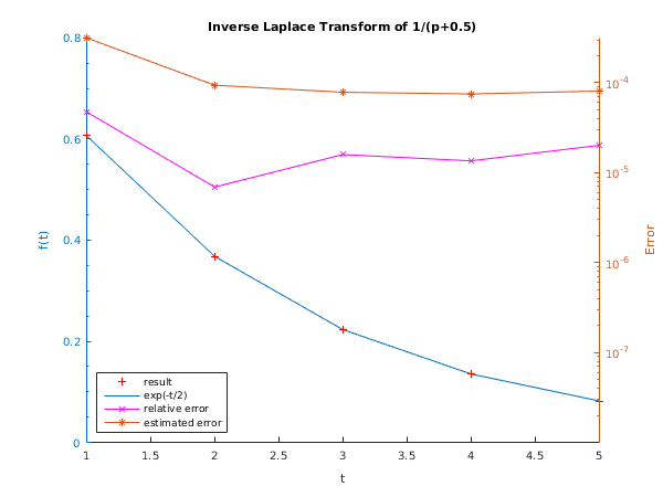
Example
This example estimates the inverse Laplace transform of the function
. The true inverse of
is
. Two preliminary calls to the function are made to verify that the chosen value of
alphab is suitable. For these tests the single value
is used. To test values of
close to
alphab, the values
and
are chosen. To test larger
, the values
and
are used. Because the values of the computed inverse are similar and
in each case, these tests show that there is unlikely to be a singularity of
in the region
.
Open in the MATLAB editor:
c06la_example
function c06la_example
fprintf('c06la example results\n\n');
mxterm = int64(200);
alphab = -0.5;
n = 1;
trures = zeros(1, n);
trurel = zeros(1, n);
t(1) = 1;
disp(['Test with t(1) = ',num2str(t(1))]);
tfac = 7.5;
relerr = 1e-2;
fprintf(['\nmxterm = %3.0f tfac = %3.2f alphab = %3.2f ', ...
'relerr = %3.0e \n\n'], mxterm,tfac,alphab,relerr);
[valinv, errest, nterms, na, alow, ahigh, nfeval, ifail] = ...
c06la( ...
@fun, t, relerr, alphab, 'tfac', tfac, 'mxterm',mxterm);
trures(1) = exp(double(-t(1)/2));
trurel(1) = abs((valinv(1)-trures(1))/trures(1));
disp('t Result exp(t/2) Relative error Error estimate')
fprintf('%1.1f %8.4f %8.4f %8.4f %8.4f\n',...
t(1), valinv(1), trures(1), trurel(1), errest(1));
fprintf(['\nnterms = %3d nfeval = %3d alow = %3.2f ', ...
'ahigh = %3.2f ifail = %3d\n\n'], nterms, nfeval, alow, ...
ahigh, ifail);
tfac = 0.8;
relerr = 1e-3;
disp(['Test with t(1) = ',num2str(t(1))]);
fprintf(['\nmxterm = %3d tfac = %3.2f alphab = %3.2f ', ...
'relerr = %3.0e \n\n'], mxterm, tfac, alphab, relerr);
[valinv, errest, nterms, na, alow, ahigh, nfeval, ifail] = ...
c06la( ...
@fun, t, relerr, alphab, 'tfac', tfac, 'mxterm',mxterm);
trures(1) = exp(double(-t(1)/2));
trurel(1) = abs((valinv(1)-trures(1))/trures(1));
disp('t Result exp(t/2) Relative error Error estimate')
fprintf('%1.1f %8.4f %8.4f %8.5f %8.5f\n',...
t(1), valinv(1), trures(1), trurel(1), errest(1));
fprintf(['\nnterms = %3d nfeval = %3d alow = %3.2f ', ...
'ahigh = %3.2f ifail = %3d\n\n'], nterms, nfeval, alow, ...
ahigh, ifail);
n = 5;
t = [1:5];
disp('Compute inverse')
fprintf(['\nmxterm = %3d tfac = %3.2f alphab = %3.2f ', ...
'relerr = %3.0e \n\n'], mxterm, tfac, alphab, relerr);
[valinv, errest, nterms, na, alow, ahigh, nfeval, ifail] = ...
c06la( ...
@fun, t, relerr, alphab, 'tfac', tfac, 'mxterm',mxterm);
disp('t Result exp(t/2) Relative error Error estimate')
for i = 1:n
trures(i) = exp(-t(i)/2);
trurel(i) = abs((valinv(i)-trures(i))/trures(i));
fprintf('%1.0f ',t(i));
fprintf(' %4.3f %4.3f %4.3e %4.3e\n',...
valinv(i),trures(i),trurel(i),errest(i));
end
fprintf(['\nmxterm = %3d tfac = %3.2f alphab = %3.2f ', ...
'relerr = %3.0e \n\n'], mxterm, tfac, alphab, relerr);
fig1 = figure;
display_plot(t,trures,valinv,trurel,errest);
function [fr,fi] = fun(preal,pimag)
z = complex(1)/complex(preal+0.5,pimag);
fr = real(z);
fi = imag(z);
function display_plot(t, trures, valinv, trurel, errest)
[haxes, hline1, hline2] = plotyy(t, valinv, t, trurel, 'plot', 'semilogy');
hold on
hpoints = plot(t, trures, '+', 'MarkerEdgeColor', 'r');
set(haxes(1), 'YLim', [0 0.8]);
set(haxes(1), 'YMinorTick', 'on');
set(haxes(1), 'YTick', [0.0 0.2 0.4 0.6 0.8]);
set(haxes(2), 'YLim', [1e-7 5e-3]);
set(haxes(2), 'YMinorTick', 'on');
set(haxes(2), 'YTick', [1e-7 1e-6 1e-5 1e-4]);
for iaxis = 1:2
set(haxes(iaxis), 'XLim', [1 5]);
set(haxes(iaxis), 'XTick', [1 1.5 2 2.5 3 3.5 4 4.5 5]);
end
set(gca, 'box', 'off');
title('Inverse Laplace Transform of 1/(p+0.5)');
xlabel('t');
ylabel(haxes(1),'f(t)');
set(haxes(2),'YLim',[1e-8 Inf]);
ylabel(haxes(2),'Error');
axes(haxes(2));
hold on;
hline3 = semilogy(t, errest);
set(hline1, 'Linewidth', 0.5, 'MarkerFaceColor', 'auto');
set(hline2, 'Linewidth', 0.5, 'Marker', 'x', 'Color','Magenta');
set(hline3, 'Linewidth', 0.5, 'Marker', '*', 'MarkerFaceColor', 'auto');
legend([hpoints hline1 hline2 hline3], 'result', 'exp(-t/2)', ...
'relative error', 'estimated error', 'Location','SouthWest');
c06la example results

Test with t(1) = 1

mxterm = 200   tfac = 7.50   alphab = -0.50 relerr = 1e-02

t     Result     exp(t/2)   Relative error   Error estimate
1.0     0.6071      0.6065        0.0010           0.0037

nterms =  18   nfeval =  36   alow = -0.04 ahigh = 0.09   ifail =   0

Test with t(1) = 1

mxterm = 200   tfac = 0.80   alphab = -0.50 relerr = 1e-03

t     Result     exp(t/2)   Relative error   Error estimate
1.0     0.6065      0.6065       0.00002          0.00008

nterms =  13   nfeval =  28   alow = 5.26 ahigh = 6.51   ifail =   0

Compute inverse

mxterm = 200   tfac = 0.80   alphab = -0.50 relerr = 1e-03

t    Result    exp(t/2)   Relative error  Error estimate
1    0.607      0.607      4.746e-05      3.155e-04
2    0.368      0.368      6.910e-06      9.386e-05
3    0.223      0.223      1.589e-05      7.839e-05
4    0.135      0.135      1.353e-05      7.504e-05
5    0.082      0.082      2.014e-05      8.080e-05

mxterm = 200   tfac = 0.80   alphab = -0.50 relerr = 1e-03
PDF version (NAG web site
, 64-bit version, 64-bit version)
© The Numerical Algorithms Group Ltd, Oxford, UK. 2009–2015