FEM Solver manual

This program solves the time dependant Laplace and Poisson equations on an arbitrary mesh by using the finite element method. The mesh is generated by using the NAG d06 routines on boundaries drawn by the user. Three different routines are available, using three different algorithms for the mesh generation: d06aa (incremental), d06ab (Delaunay) and d06ac (Advancing front). d06ba is also used to subdivide the boundaries. The linear system is solved using the f11 routines: f11zb (renumbering), f11ja (preconditioning) and f11jc (solving). The user can set boundary conditions, choose the time parameters and export the results of the simulation.

The interface is divided in 6 parts: the drawing area, the toolbar, the boundaries list, the algorithm selector, the equations buttons and the help text area.

Fig 1 - Overview

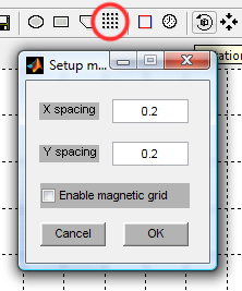
The drawing area allows the user to draw the domain on which he wants to solve the equations. It's also the place where the solution is displayed. In the drawing mode, the user can add boundaries using three different tools (circle, rectangle and polylines). A grid is available to help the user drawing straight lines, it can be configured through the toolbar button. In the visualisation mode, several tools are available to see the solutions in different angles and drawing modes by using the toolbar.

• 
  File management
• 
  Drawing tools: circle, rectangle and polylines
• 
  Setup magnetic grid for the drawing area
• 
  Setup boundary conditions
• 
  Change the time parameters of the simulation
• 
  3D rotation of the solution
• 
  Reset the top view
• 
  Zoom in/out
• 
  Pan
• 
  Configures axes
• 
  Data cursor to read the coordinates of a point
• 
  Colormap editor
• 
  Activate/Deactivate the elements outline
• 
  Activate/Deactivate the grid on the solution
• 
  Activate/Deactivate the boundary condition labels on the domain
• 
  Solution display control: start, pause and stop
• 
  Save the video of the solution in matlab format

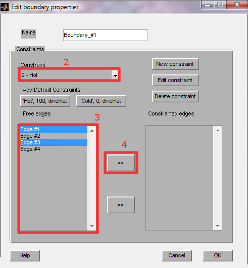
The user can delete or edit the boundaries of the selected domain. When editing a boundary, the user can change its name and decide to apply different conditions on each edge of the boundary.

The user can choose which algorithm to use to generate the mesh and can configure each algorithm separately.

The program solves the chosen equation when the user clicks on the buttons. For the poisson equation the user has to enter the source term.

In all the expressions (initial value, source term or conditions) the syntax is checked. The user can use 3 variables in these expressions: x, y and t for the current point coordinates and time. Every correct matlab expression using only these variables (or none) are allowed.

All the program settings are saved in a XML file named config.xml.

This tutorial will demonstrate how to configure the drawing area. The following tutorials will use the same configuration.

1. Select the Magnetic grid tool to open the grid configuration dialog. Enter the values [0.5;0.5] for the grid step. If 'enable' is checked, then all vertices of boundaries will snap to the grid.
   
   Fig 2 - Grid configuration
2. Select the Axes configuration tool to open the configuration dialog. Enter the values [-1.5;1.5] for the axes limits.
   
   Fig 3 - Axes configuration

This tutorial demonstrates how to use the polyline tool.

1. Select the polyline tool.
2. Left click in the drawing area to place the first vertex of the polygon.
3. Continue placing the vertices of the polygon in an anticlockwise fashion using the left mouse button.
4. When you wish to complete the polygon, place the final vertex by clicking with the right mouse button instead of the left.

   WARNING: Do not cross the lines of the polygon or click twice on the same vertex, as this will result in an error!

Fig 4 - Drawing a polygon domain

1. If you wish to create a hole in your domain, then click the polyline tool again.
2. Left click within the current boundary in which you wish to create a hole.
3. Continue placing vertices with the left mouse button,this time in a clockwise direction.
4. Place the final vertex with the right mouse button.

Fig 5 - Creating a polygon hole in a domain

This tutorial will demonstrate how to use the basic functions of the program to solve the Laplace equation on a square.

The first thing to do is to draw the domain we want to solve the problem into. This is done in 5 steps (assuming you have already configured the drawing area).

1. Choose the Incremental algorithm in the algorithms list.
2. Click on the rectangle tool.
3. Click on the first corner (-1,1).
4. Click on the second corner (1,-1).

Fig 4 - Drawing the domain

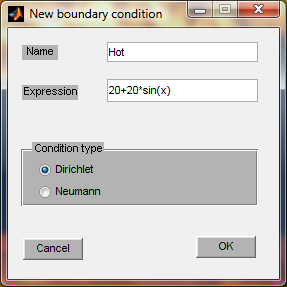
Now we have to add some boundary conditions

1. Click on the New condition tool . A dialog will show up
2. Add a cold condition named 'Cold' and with '0' as expression
   
   Fig 5 - Cold condition
   Press the 'OK' button to finish creating the condition.

   NB: If you wish to edit the condition, click on Edit in the Boundaries panel, select the condition from the drop down list, and click 'Edit constraint'. Make your changes and click OK.

3. Add a hot condition named 'hot' and with '20 + 20*sin(x)' as expression
   
   Fig 6 - Hot condition
   Press OK to finish creating the condition.

Then we assign the conditions to the boundary edges

1. Click on the edit button from the boundaries list, a dialog will show up
2. Select the 'hot' condition from the list
3. Select edge 1 and 3 (holding ctrl key) from the free edges list on the left
   
4. Click on the '>>' button to assign the hot condition to these edges. They should be on the right list
   
5. Click ok to return

Now we change the time parameters

1. Click on the time configuration tool in the toolbar
2. Change the parameters with dt=0.1 and T=5
   
   Fig 7 - Time configuration
   Then click ok

Everything is ready we can now hit the 'Laplace' button. You will be asked the initial value, leave '0'. When the solving is finished you can watch the solution by clicking on the play button from the toolbar. At the end of the animation you should see the steady state as in Fig 8.

Fig 8 - Steady state