PDF version (NAG web site
, 64-bit version, 64-bit version)
NAG Toolbox: nag_pde_1d_blackscholes_fd (d03nc)
Purpose
nag_pde_1d_blackscholes_fd (d03nc) solves the Black–Scholes equation for financial option pricing using a finite difference scheme.
Syntax
[
s,
t,
f,
theta,
delta,
gamma,
lambda,
rho,
ifail] = d03nc(
kopt,
x,
mesh,
s,
t,
tdpar,
r,
q,
sigma,
ntkeep, 'ns',
ns, 'nt',
nt, 'alpha',
alpha)
[
s,
t,
f,
theta,
delta,
gamma,
lambda,
rho,
ifail] = nag_pde_1d_blackscholes_fd(
kopt,
x,
mesh,
s,
t,
tdpar,
r,
q,
sigma,
ntkeep, 'ns',
ns, 'nt',
nt, 'alpha',
alpha)
Description
nag_pde_1d_blackscholes_fd (d03nc) solves the Black–Scholes equation (see
Hull (1989) and
Wilmott et al. (1995))
for the value
of a European or American, put or call stock option, with exercise price
. In equation
(1) is time,
is the stock price,
is the risk free interest rate,
is the continuous dividend, and
is the stock volatility. According to the values in the array
tdpar, the arguments
,
and
may each be either constant or functions of time. The function also returns values of various Greeks.
nag_pde_1d_blackscholes_fd (d03nc) uses a finite difference method with a choice of time-stepping schemes. The method is explicit for
and implicit for nonzero values of
alpha. Second order time accuracy can be obtained by setting
. According to the value of the argument
mesh the finite difference mesh may be either uniform, or user-defined in both
and
directions.
References
Hull J (1989) Options, Futures and Other Derivative Securities Prentice–Hall
Wilmott P, Howison S and Dewynne J (1995) The Mathematics of Financial Derivatives Cambridge University Press
Parameters
Compulsory Input Parameters
- 1:
– int64int32nag_int scalar
-
Specifies the kind of option to be valued.
- A European call option.
- An American call option.
- A European put option.
- An American put option.
Constraint:
, , or .
- 2:
– double scalar
-
The exercise price .
- 3:
– string (length ≥ 1)
-
Indicates the type of finite difference mesh to be used:
- Uniform mesh.
- Custom mesh supplied by you.
Constraint:
or .
- 4:
– double array
-
If
,
must contain the
th stock price in the mesh, for
. These values should be in increasing order, with
and
.
If , must be set to and to , but need not be initialized, as they will be set internally by the function in order to define a uniform mesh.
Constraints:
- if , and , for ;
- if , .
- 5:
– double array
-
If
then
must contain the
th time in the mesh, for
. These values should be in increasing order, with
and
.
If then must be set to and to , but need not be initialized, as they will be set internally by the function in order to define a uniform mesh.
Constraints:
- if , and , for ;
- if , .
- 6:
– logical array
-
Specifies whether or not various arguments are time-dependent. More precisely, is time-dependent if and constant otherwise. Similarly, specifies whether is time-dependent and specifies whether is time-dependent.
- 7:
– double array
-
The dimension of the array
r
must be at least
if
, and at least
otherwise
If
then
must contain the value of the risk-free interest rate
at the
th time in the mesh, for
.
If then must contain the constant value of the risk-free interest rate . The remaining elements need not be set.
- 8:
– double array
-
The dimension of the array
q
must be at least
if
, and at least
otherwise
If
then
must contain the value of the continuous dividend
at the
th time in the mesh, for
.
If then must contain the constant value of the continuous dividend . The remaining elements need not be set.
- 9:
– double array
-
The dimension of the array
sigma
must be at least
if
, and at least
otherwise
If
then
must contain the value of the volatility
at the
th time in the mesh, for
.
If then must contain the constant value of the volatility . The remaining elements need not be set.
- 10:
– int64int32nag_int scalar
-
The number of solutions to be stored in the time direction. The function calculates the solution backwards from
to
at all times in the mesh. These time solutions and the corresponding Greeks will be stored at times
, for
, in the arrays
f,
theta,
delta,
gamma,
lambda and
rho. Other time solutions will be discarded. To store all time solutions set
.
Constraint:
.
Optional Input Parameters
- 1:
– int64int32nag_int scalar
-
Default:
the dimension of the array
s.
The number of stock prices to be used in the finite difference mesh.
Constraint:
.
- 2:
– int64int32nag_int scalar
-
Default:
the dimension of the array
t.
The number of time-steps to be used in the finite difference method.
Constraint:
.
- 3:
– double scalar
Default:
The value of
to be used in the time-stepping scheme. Typical values include:
- Explicit forward Euler scheme.
- Implicit Crank–Nicolson scheme.
- Implicit backward Euler scheme.
The value gives second-order accuracy in time. Values greater than give unconditional stability. Since is at the limit of unconditional stability this value does not damp oscillations.
Constraint:
.
Output Parameters
- 1:
– double array
-
If
, the elements of
s define a uniform mesh over
.
If
, the elements of
s are unchanged.
- 2:
– double array
-
If
, the elements of
t define a uniform mesh over
.
If
, the elements of
t are unchanged.
- 3:
– double array
-
, for and , contains the value of the option at the th mesh point at time .
- 4:
– double array
- 5:
– double array
- 6:
– double array
- 7:
– double array
- 8:
– double array
-
The values of various Greeks at the
th mesh point
at time
, as follows:
- 9:
– int64int32nag_int scalar
unless the function detects an error (see
Error Indicators and Warnings).
Error Indicators and Warnings
Errors or warnings detected by the function:
-
-
| On entry, | , |
| or | , |
| or | or , |
| or | , |
| or | , |
| or | , |
| or | , |
| or | , |
| or | , |
| or | , |
| or | , |
| or | . |
-
-
and the constraints:
are violated. Thus the end points of the uniform mesh are not in order.
-
-
and the constraints:
- , for ,
- , for
are violated. Thus the mesh points are not in order.
-
An unexpected error has been triggered by this routine. Please
contact
NAG.
-
Your licence key may have expired or may not have been installed correctly.
-
Dynamic memory allocation failed.
Accuracy
The accuracy of the solution
and the various derivatives returned by the function is dependent on the values of
ns and
nt supplied, the distribution of the mesh points, and the value of
alpha chosen. For most choices of
alpha the solution has a truncation error which is second-order accurate in
and first order accurate in
. For
the truncation error is also second-order accurate in
.
The simplest approach to improving the accuracy is to increase the values of both
ns and
nt.
Further Comments
Timing
Each time-step requires the construction and solution of a tridiagonal system of linear equations. To calculate each of the derivatives
lambda and
rho requires a repetition of the entire solution process. The time taken for a call to the function is therefore proportional to
.
Algorithmic Details
nag_pde_1d_blackscholes_fd (d03nc) solves equation
(1) using a finite difference method. The solution is computed backwards in time from
to
using a
scheme, which is implicit for all nonzero values of
, and is unconditionally stable for values of
. For each time-step a tridiagonal system is constructed and solved to obtain the solution at the earlier time. For the explicit scheme (
) this tridiagonal system degenerates to a diagonal matrix and is solved trivially. For American options the solution at each time-step is inspected to check whether early exercise is beneficial, and amended accordingly.
To compute the arrays
lambda and
rho, which are derivatives of the stock value
with respect to the problem arguments
and
respectively, the entire solution process is repeated with perturbed values of these arguments.
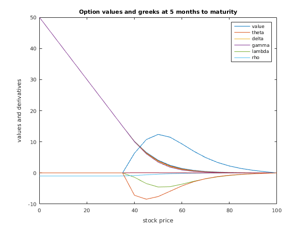
Example
This example, taken from
Hull (1989), solves the one-dimensional Black–Scholes equation for valuation of a
-month American put option on a non-dividend-paying stock with an exercise price of $50. The risk-free interest rate is 10% per annum, and the stock volatility is 40% per annum.
A fully implicit backward Euler scheme is used, with a mesh of stock price intervals and time intervals.
Open in the MATLAB editor:
d03nc_example
function d03nc_example
fprintf('d03nc example results\n\n');
kopt = int64(4);
x = 50;
mesh = 'U';
n = 21;
nt = 11;
s = zeros(n,1);
s(n) = 100;
t = zeros(nt,1);
t(nt) = 0.4166667;
tdpar = [false; false; false];
r = [0.1];
q = [0];
sigma = [0.4];
ntkeep = int64(4);
alpha = 1;
[s, t, f, theta, delta, gamma, lambda, rho, ifail] = ...
d03nc(...
kopt, x, mesh, s, t, tdpar, r, q, sigma, ntkeep,'alpha',alpha);
disp(' Option Values');
disp(' Stock Price | Time to Maturity (months)');
fprintf('%16s','|');
fprintf('%12.1f',12*(t(nt)-t(1:ntkeep)));
fprintf('\n');
for i = 1:n
fprintf('%12.0f%4s', s(i), '|');
fprintf(' %12.5f', f(i,:));
fprintf('\n');
end
fig1 = figure;
plot(s,f,s,theta(:,1),s,delta(:,1),s,gamma(:,1),s,...
lambda(:,1),s,rho(:,1));
legend('value','theta','delta','gamma','lambda','rho');
title('Option values and greeks at 5 months to maturity');
xlabel('stock price');
ylabel('values and derivatives');
d03nc example results

         Option Values
  Stock Price  |   Time to Maturity (months)
               |         5.0         4.5         4.0         3.5
           0   |     50.00000     50.00000     50.00000     50.00000
           5   |     45.00000     45.00000     45.00000     45.00000
          10   |     40.00000     40.00000     40.00000     40.00000
          15   |     35.00000     35.00000     35.00000     35.00000
          20   |     30.00000     30.00000     30.00000     30.00000
          25   |     25.00000     25.00000     25.00000     25.00000
          30   |     20.00000     20.00000     20.00000     20.00000
          35   |     15.00000     15.00000     15.00000     15.00000
          40   |     10.15432     10.09580     10.04640     10.01169
          45   |      6.58481      6.44237      6.29161      6.13058
          50   |      4.06719      3.87850      3.67292      3.44630
          55   |      2.42637      2.24235      2.04536      1.83361
          60   |      1.41742      1.26619      1.10958      0.94813
          65   |      0.81951      0.70724      0.59532      0.48515
          70   |      0.47241      0.39411      0.31904      0.24845
          75   |      0.27257      0.22016      0.17174      0.12815
          80   |      0.15725      0.12328      0.09294      0.06668
          85   |      0.08966      0.06848      0.05010      0.03473
          90   |      0.04845      0.03625      0.02590      0.01747
          95   |      0.02110      0.01558      0.01097      0.00727
         100   |      0.00000      0.00000      0.00000      0.00000
PDF version (NAG web site
, 64-bit version, 64-bit version)
© The Numerical Algorithms Group Ltd, Oxford, UK. 2009–2015