PDF version (NAG web site
, 64-bit version, 64-bit version)
NAG Toolbox: nag_pde_3d_ellip_fd (d03ec)
Purpose
nag_pde_3d_ellip_fd (d03ec) uses the Strongly Implicit Procedure to calculate the solution to a system of simultaneous algebraic equations of seven-point molecule form on a three-dimensional topologically-rectangular mesh. (‘Topological’ means that a polar grid, for example, can be used if it is equivalent to a rectangular box.)
Syntax
[
t,
itcoun,
itused,
resids,
chngs,
ifail] = d03ec(
n1,
n2,
n3,
a,
b,
c,
d,
e,
f,
g,
q,
t,
aparam,
itmax,
itcoun,
ndir,
ixn,
iyn,
izn,
conres,
conchn, 'sda',
sda)
[
t,
itcoun,
itused,
resids,
chngs,
ifail] = nag_pde_3d_ellip_fd(
n1,
n2,
n3,
a,
b,
c,
d,
e,
f,
g,
q,
t,
aparam,
itmax,
itcoun,
ndir,
ixn,
iyn,
izn,
conres,
conchn, 'sda',
sda)
Description
Given a set of simultaneous equations
(which could be nonlinear) derived, for example, from a finite difference representation of a three-dimensional elliptic partial differential equation and its boundary conditions, the function determines the values of the dependent variable
.
is a square
by
matrix and
is a known vector of length
.
The equations must be of seven-diagonal form:
for
,
and
, provided that
.
Indeed, if
, then the equation is assumed to be:
The system is solved iteratively from a starting approximation
by the formulae:
Thus
is the residual of the
th approximate solution
, and
is the update change vector.
The calling program supplies an initial approximation for the values of the dependent variable in the array
t, the coefficients of the seven-point molecule system of equations in the arrays
a,
b,
c,
d,
e,
f and
g, and the source terms in the array
q. The function derives the residual of the latest approximate solution, and then uses the approximate
factorization of the Strongly Implicit Procedure with the necessary acceleration argument adjustment by calling
nag_pde_3d_ellip_fd_iter (d03ub) at each iteration.
nag_pde_3d_ellip_fd (d03ec) combines the newly derived change with the old approximation to obtain the new approximate solution for
. The new solution is checked for convergence against the user-supplied convergence criteria, and if these have not been satisfied, the iterative cycle is repeated. Convergence is based on both the maximum absolute normalized residuals (calculated with reference to the previous approximate solution as these are calculated at the commencement of each iteration) and on the maximum absolute change made to the values of
.
Problems in topologically non-rectangular-box-shaped regions can be solved using the function by surrounding the region by a circumscribing topologically rectangular box. The equations for the nodal values external to the region of interest are set to zero (i.e., ) and the boundary conditions are incorporated into the equations for the appropriate nodes.
If there is no better initial approximation when starting the iterative cycle, one can use an array of zeros as the initial approximation.
The function can be used to solve linear elliptic equations in which case the arrays
a,
b,
c,
d,
e,
f,
g and
q remain constant and for which a single call provides the required solution. It can also be used to solve nonlinear elliptic equations, in which case some or all of these arrays may require updating during the progress of the iterations as more accurate solutions are derived. The function will then have to be called repeatedly in an outer iterative cycle. Dependent on the nonlinearity, some under-relaxation of the coefficients and/or source terms may be needed during their recalculation using the new estimates of the solution.
The function can also be used to solve each step of a time-dependent parabolic equation in three space dimensions. The solution at each time step can be expressed in terms of an elliptic equation if the Crank–Nicolson or other form of implicit time integration is used.
Neither diagonal dominance, nor positive-definiteness, of the matrix
formed from the arrays
a,
b,
c,
d,
e,
f and
g is necessary to ensure convergence.
For problems in which the solution is not unique in the sense that an arbitrary constant can be added to the solution (for example Poisson's equation with all Neumann boundary conditions), a argument is incorporated so that the solution can be rescaled. A specified nodal value is subtracted from the whole solution after the completion of every iteration. This keeps rounding errors to a minimum for those cases when convergence is slow. For such problems there is generally an associated compatibility condition. For the example mentioned this compatibility condition equates the total net source within the region (i.e., the source integrated over the region) with the total net outflow across the boundaries defined by the Neumann conditions (i.e., the normal derivative integrated along the whole boundary). It is very important that the algebraic equations derived to model such a problem implement accurately the compatibility condition. If they do not, a net source or sink is very likely to be represented by the set of algebraic equations and no steady-state solution of the equations exists.
References
Jacobs D A H (1972) The strongly implicit procedure for the numerical solution of parabolic and elliptic partial differential equations Note RD/L/N66/72 Central Electricity Research Laboratory
Stone H L (1968) Iterative solution of implicit approximations of multi-dimensional partial differential equations SIAM J. Numer. Anal. 5 530–558
Weinstein H G, Stone H L and Kwan T V (1969) Iterative procedure for solution of systems of parabolic and elliptic equations in three dimensions Industrial and Engineering Chemistry Fundamentals 8 281–287
Parameters
Compulsory Input Parameters
- 1:
– int64int32nag_int scalar
-
The number of nodes in the first coordinate direction, .
Constraint:
.
- 2:
– int64int32nag_int scalar
-
The number of nodes in the second coordinate direction, .
Constraint:
.
- 3:
– int64int32nag_int scalar
-
The number of nodes in the third coordinate direction, .
Constraint:
.
- 4:
– double array
-
lda, the first dimension of the array, must satisfy the constraint
.
must contain the coefficient of
in the
th equation of the system
(1), for
,
and
. The elements of
a, for
, must be zero after incorporating the boundary conditions, since they involve nodal values from outside the box.
- 5:
– double array
-
lda, the first dimension of the array, must satisfy the constraint
.
must contain the coefficient of
in the
th equation of the system
(1), for
,
and
. The elements of
b, for
, must be zero after incorporating the boundary conditions, since they involve nodal values from outside the box.
- 6:
– double array
-
lda, the first dimension of the array, must satisfy the constraint
.
must contain the coefficient of
in the
th equation of the system
(1), for
,
and
. The elements of
c, for
, must be zero after incorporating the boundary conditions, since they involve nodal values from outside the box.
- 7:
– double array
-
lda, the first dimension of the array, must satisfy the constraint
.
must contain the coefficient of
(the ‘central’ term) in the
th equation of the system
(1), for
,
and
. The elements of
d are checked to ensure that they are nonzero. If any element is found to be zero, the corresponding algebraic equation is assumed to be
. This feature can be used to define the equations for nodes at which, for example, Dirichlet boundary conditions are applied, or for nodes external to the problem of interest. Setting
at appropriate points, and the corresponding value of
to the appropriate value, namely the prescribed value of
in the Dirichlet case, or to zero at an external point.
- 8:
– double array
-
lda, the first dimension of the array, must satisfy the constraint
.
must contain the coefficient of
in the
th equation of the system
(1), for
,
and
. The elements of
e, for
, must be zero after incorporating the boundary conditions, since they involve nodal values from outside the box.
- 9:
– double array
-
lda, the first dimension of the array, must satisfy the constraint
.
must contain the coefficient of
in the
th equation of the system
(1), , for
,
and
. The elements of
f, for
, must be zero after incorporating the boundary conditions, since they involve nodal values from outside the box.
- 10:
– double array
-
lda, the first dimension of the array, must satisfy the constraint
.
must contain the coefficient of
in the
th equation of the system
(1), for
,
and
. The elements of
g, for
, must be zero after incorporating the boundary conditions, since they involve nodal values from outside the box.
- 11:
– double array
-
lda, the first dimension of the array, must satisfy the constraint
.
must contain
, for
,
and
, i.e., the source-term values at the nodal points of the system
(1).
- 12:
– double array
-
lda, the first dimension of the array, must satisfy the constraint
.
must contain the element
of an approximate solution to the equations, for
,
and
.
If no better approximation is known, an array of zeros can be used.
- 13:
– double scalar
-
The iteration acceleration factor. A value of is adequate for most typical problems. However, if convergence is slow, the value can be reduced, typically to or . If divergence is obtained, the value can be increased, typically to , or .
Constraint:
.
- 14:
– int64int32nag_int scalar
-
The maximum number of iterations to be used by the function in seeking the solution. A reasonable value might be for a problem with nodes and convergence criteria of about of the original residual and change.
- 15:
– int64int32nag_int scalar
-
On the first call of
nag_pde_3d_ellip_fd (d03ec),
itcoun must be set to
. On subsequent entries, its value must be unchanged from the previous call.
- 16:
– int64int32nag_int scalar
-
Indicates whether or not the system of equations has a unique solution. For systems which have a unique solution,
ndir must be set to any nonzero value. For systems derived from problems to which an arbitrary constant can be added to the solution, for example Poisson's equation with all Neumann boundary conditions,
ndir should be set to
and the values of the next three arguments must be specified. For such problems the function subtracts the value of the function derived at the node (
ixn,
iyn,
izn) from the whole solution after each iteration to reduce the possibility of large rounding errors. You must also ensure for such problems that the appropriate compatibility condition on the source terms
q is satisfied. See the comments at the end of
Description.
- 17:
– int64int32nag_int scalar
-
Is ignored unless
ndir is equal to zero, in which case it must specify the first index of the nodal point at which the solution is to be set to zero. The node should not correspond to a corner node, or to a node external to the region of interest.
- 18:
– int64int32nag_int scalar
-
Is ignored unless
ndir is equal to zero, in which case it must specify the second index of the nodal point at which the solution is to be set to zero. The node should not correspond to a corner node, or to a node external to the region of interest.
- 19:
– int64int32nag_int scalar
-
Is ignored unless
ndir is equal to zero, in which case it must specify the third index of the nodal point at which the solution is to be set to zero. The node should not correspond to a corner node, or to a node external to the region of interest.
- 20:
– double scalar
-
The convergence criterion to be used on the maximum absolute value of the normalized residual vector components. The latter is defined as the residual of the algebraic equation divided by the central coefficient when the latter is not equal to
, and defined as the residual when the central coefficient is zero.
conres should not be less than a reasonable multiple of the
machine precision.
- 21:
– double scalar
-
The convergence criterion to be used on the maximum absolute value of the change made at each iteration to the elements of the array
t, namely the dependent variable.
conchn should not be less than a reasonable multiple of the machine accuracy multiplied by the maximum value of
t attained.
Convergence is achieved when both the convergence criteria are satisfied. You can therefore set convergence on either the residual or on the change, or (as is recommended) on a requirement that both are below prescribed limits.
Optional Input Parameters
- 1:
– int64int32nag_int scalar
-
Default:
the second dimension of the arrays
a,
b,
c,
d,
e,
f,
g,
q,
t. (An error is raised if these dimensions are not equal.)
The second dimension of the arrays
a,
b,
c,
d,
e,
f,
g,
q,
t,
wrksp1,
wrksp2,
wrksp3 and
wrksp4.
Constraint:
.
Output Parameters
- 1:
– double array
-
The solution derived by the function.
- 2:
– int64int32nag_int scalar
-
Its value is increased by the number of iterations used on this call (namely
itused). It therefore stores the accumulated number of iterations actually used.
For subsequent calls for the same problem, i.e., with the same
n1,
n2 and
n3 but possibly different coefficients and/or source terms, as occur with nonlinear systems or with time-dependent systems,
itcoun should not be reset, i.e., it must contain the accumulated number of iterations. In this way a suitable cycling of the sequence of iteration arguments is obtained in the calls to
nag_pde_3d_ellip_fd_iter (d03ub).
- 3:
– int64int32nag_int scalar
-
The number of iterations actually used on that call.
- 4:
– double array
-
The maximum absolute value of the residuals calculated at the
th iteration, for
. If the residual of the solution is sought you must calculate this in the function from which
nag_pde_3d_ellip_fd (d03ec) is called. The sequence of values
resids indicates the rate of convergence.
- 5:
– double array
-
The maximum absolute value of the changes made to the components of the dependent variable
t at the
th iteration, for
. The sequence of values
chngs indicates the rate of convergence.
- 6:
– int64int32nag_int scalar
unless the function detects an error (see
Error Indicators and Warnings).
Error Indicators and Warnings
Note: nag_pde_3d_ellip_fd (d03ec) may return useful information for one or more of the following detected errors or warnings.
Errors or warnings detected by the function:
-
-
| On entry, | , |
| or | , |
| or | . |
-
-
| On entry, | , |
| or | . |
-
-
-
-
| On entry, | . |
-
-
Convergence was not achieved after
itmax iterations.
-
An unexpected error has been triggered by this routine. Please
contact
NAG.
-
Your licence key may have expired or may not have been installed correctly.
-
Dynamic memory allocation failed.
Accuracy
The improvement in accuracy for each iteration depends on the size of the system and on the condition of the update matrix characterised by the seven-diagonal coefficient arrays. The ultimate accuracy obtainable depends on the above factors and on the
machine precision. The rate of convergence obtained with the Strongly Implicit Procedure is not always smooth because of the cyclic use of nine acceleration arguments. The convergence may become slow with very large problems. The final accuracy obtained may be judged approximately from the rate of convergence determined from the sequence of values returned in the arrays
resids and
chngs and the magnitude of the maximum absolute value of the change vector on the last iteration stored in
.
Further Comments
The time taken per iteration is approximately proportional to .
Convergence may not always be obtained when the problem is very large and/or the coefficients of the equations have widely disparate values. The latter case is often associated with a near ill-conditioned matrix.
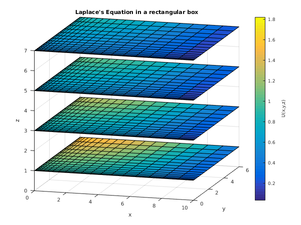
Example
This example solves Laplace's equation in a rectangular box with a non-uniform grid spacing in the
,
, and
coordinate directions and with Dirichlet boundary conditions specifying the function on the surfaces of the box equal to
Note that this is the same problem as that solved in the example for
nag_pde_3d_ellip_fd_iter (d03ub). The differences in the maximum residuals obtained at each iteration between the two test runs are explained by the fact that in
nag_pde_3d_ellip_fd (d03ec) the residual at each node is normalized by dividing by the central coefficient, whereas this normalization has not been used in the example program for
nag_pde_3d_ellip_fd_iter (d03ub).
Open in the MATLAB editor:
d03ec_example
function d03ec_example
fprintf('d03ec example results\n\n');
n1 = int64(16);
n2 = int64(20);
n3 = int64(24);
a = zeros(n1, n2, n3);
b = a; c = a; c = a; e = a; f = a; g = a; q = a; u0 = a;
aparam = 1;
itmax = int64(100); itcoun = int64(0); ndir = int64(1);
ixn = int64(0); iyn = ixn; izn = ixn;
conres = 1e-06; conchn = 1e-06;
delta = 12.0/double(n1*(n1-1));
for i = 1:n1
x(i) = delta*double(i*(i-1))/2;
end
delta = 20.0/double(n2*(n2-1));
for i = 1:n2
y(i) = delta*double(i*(i-1))/2;
end
delta = 30.0/double(n3*(n3-1));
for i = 1:n3
z(i) = delta*double(i*(i-1))/2;
end
for k = 2:n3-1
a(2:n1-1,2:n2-1,k) = 2/((z(k)-z(k-1))*(z(k+1)-z(k-1)));
g(2:n1-1,2:n2-1,k) = 2/((z(k+1)-z(k))*(z(k+1)-z(k-1)));
end
for j = 2:n2-1
b(2:n1-1,j,2:n3-1) = 2/((y(j)-y(j-1))*(y(j+1)-y(j-1)));
f(2:n1-1,j,2:n3-1) = 2/((y(j+1)-y(j))*(y(j+1)-y(j-1)));
end
for i = 2:n1-1
c(i,2:n2-1,2:n3-1) = 2/((x(i)-x(i-1))*(x(i+1)-x(i-1)));
e(i,2:n2-1,2:n3-1) = 2/((x(i+1)-x(i))*(x(i+1)-x(i-1)));
end
d = - a - b - c - e - f - g;
scale = 1/y(n2);
exact = @(x,y,z)(exp((x+1)*scale)* cos(sqrt(2)*y*scale)* exp((-z-1)*scale));
q(1, 1:n2, 1:n3) = exact(x(1), y', z);
q(n1, 1:n2, 1:n3) = exact(x(n1),y', z);
q(1:n1,1 , 1:n3) = exact(x', y(1), z);
q(1:n1,n2 , 1:n3) = exact(x', y(n2),z);
q(1:n1,1:n2, 1) = exact(x', y, z(1));
q(1:n1,1:n2, n3) = exact(x', y, z(n3));
[u, itcoun, itused, resids, chngs, ifail] = ...
d03ec( ...
n1, n2, n3, a, b, c, d, e, f, g, q, u0, aparam, itmax, itcoun, ...
ndir, ixn, iyn, izn, conres, conchn);
fprintf('Number of iterations %4d\n',itused);
fprintf('Maximum residual %8.3e\n',resids(itused));
fig1 = figure;
[xs,ys,zs] = meshgrid(y,x,z);
slice(xs,ys,zs,u,[],[],double([1 3 5 7]));
axis([y(1) y(end) x(1) x(end) 0 7]);
xlabel('x'); ylabel('y'); zlabel('z');
title('Laplace''s Equation in a rectangular box');
view(16, 14);
h = colorbar;
ylabel(h, 'U(x,y,z)')
d03ec example results

Number of iterations    12
Maximum residual       1.193e-07
PDF version (NAG web site
, 64-bit version, 64-bit version)
© The Numerical Algorithms Group Ltd, Oxford, UK. 2009–2015