d02pd:: Ordinary Differential EquationsIntegrators for Stiff Ordinary Differential Systems (NAG Toolbox)

nag_ode_ivp_rk_onestep (d02pd) and its associated functions (nag_ode_ivp_rk_setup (d02pv), nag_ode_ivp_rk_reset_tend (d02pw), nag_ode_ivp_rk_interp (d02px), nag_ode_ivp_rk_diag (d02py) and nag_ode_ivp_rk_errass (d02pz)) solve an initial value problem for a first-order system of ordinary differential equations. The functions, based on Runge–Kutta methods and derived from RKSUITE (see Brankin et al. (1991)), integrate

y^{'} = f (t, y) given y (t_{0}) = y_{0}

where

y

is the vector of

n

solution components and

t

is the independent variable.

nag_ode_ivp_rk_onestep (d02pd) is designed to be used in complicated tasks when solving systems of ordinary differential equations. You must first call nag_ode_ivp_rk_setup (d02pv) to specify the problem and how it is to be solved. Thereafter you (repeatedly) call nag_ode_ivp_rk_onestep (d02pd) to take one integration step at a time from tstart in the direction of tend (as specified in nag_ode_ivp_rk_setup (d02pv)). In this manner nag_ode_ivp_rk_onestep (d02pd) returns an approximation to the solution ynow and its derivative ypnow at successive points tnow. If nag_ode_ivp_rk_onestep (d02pd) encounters some difficulty in taking a step, the integration is not advanced and the function returns with the same values of tnow, ynow and ypnow as returned on the previous successful step. nag_ode_ivp_rk_onestep (d02pd) tries to advance the integration as far as possible subject to passing the test on the local error and not going past tend.

In the call to nag_ode_ivp_rk_setup (d02pv) you can specify either the first step size for nag_ode_ivp_rk_onestep (d02pd) to attempt or that it compute automatically an appropriate value. Thereafter nag_ode_ivp_rk_onestep (d02pd) estimates an appropriate step size for its next step. This value and other details of the integration can be obtained after any call to nag_ode_ivp_rk_onestep (d02pd) by a call to nag_ode_ivp_rk_diag (d02py). The local error is controlled at every step as specified in nag_ode_ivp_rk_setup (d02pv). If you wish to assess the true error, you must set

errass = true

in the call to nag_ode_ivp_rk_setup (d02pv). This assessment can be obtained after any call to nag_ode_ivp_rk_onestep (d02pd) by a call to nag_ode_ivp_rk_errass (d02pz).

If you want answers at specific points there are two ways to proceed:

(i)

The more efficient way is to step past the point where a solution is desired, and then call nag_ode_ivp_rk_interp (d02px) to get an answer there. Within the span of the current step, you can get all the answers you want at very little cost by repeated calls to nag_ode_ivp_rk_interp (d02px). This is very valuable when you want to find where something happens, e.g., where a particular solution component vanishes. You cannot proceed in this way with

method = 3

(ii)

The other way to get an answer at a specific point is to set tend to this value and integrate to tend. nag_ode_ivp_rk_onestep (d02pd) will not step past tend, so when a step would carry it past, it will reduce the step size so as to produce an answer at tend exactly. After getting an answer there (

tnow = tend

), you can reset tend to the next point where you want an answer, and repeat. tend could be reset by a call to nag_ode_ivp_rk_setup (d02pv), but you should not do this. You should use nag_ode_ivp_rk_reset_tend (d02pw) instead because it is both easier to use and much more efficient. This way of getting answers at specific points can be used with any of the available methods, but it is the only way with

method = 3

. It can be inefficient. Should this be the case, the code will bring the matter to your attention.

References

Parameters

Compulsory Input Parameters

Optional Input Parameters

Output Parameters

Error Indicators and Warnings

Cases prefixed with W are classified as warnings and do not generate an error of type NAG:error_n. See nag_issue_warnings.

Accuracy

Further Comments

If nag_ode_ivp_rk_onestep (d02pd) returns with

ifail = 5

and the accuracy specified by tol and thres is really required then you should consider whether there is a more fundamental difficulty. For example, the solution may contain a singularity. In such a region the solution components will usually be large in magnitude. Successive output values of ynow should be monitored with the aim of trapping the solution before the singularity. In any case numerical integration cannot be continued through a singularity, and analytical treatment may be necessary.

Example

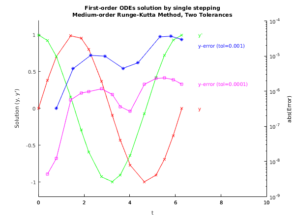
This example solves the equation

y^{''} = - y, y (0) = 0, y^{'} (0) = 1

reposed as

y_{1}^{'} = y_{2}

y_{2}^{'} = - y_{1}

over the range

[0, 2 π]

with initial conditions

y_{1} = 0.0

and

y_{2} = 1.0

. We use relative error control with threshold values of

1.0e−8

for each solution component and print the solution at each integration step across the range. We use a medium order Runge–Kutta method (

method = 2

) with tolerances

tol = 1.0e−4

and

tol = 1.0e−5

in turn so that we may compare the solutions. The value of

π

is obtained by using nag_math_pi (x01aa).

function d02pd_example


fprintf('d02pd example results\n\n');

% Set initial conditions and input
method = int64(2);
tstart = 0;
tend   = 2*pi;
n      = int64(2);
errass = false;
lenwrk = int64(32*n);
yinit  = [0;1];
hstart = 0;
thresh = [1e-08; 1e-08];
ynow = zeros(20, n);
tnow = zeros(20, 1);
err1 = zeros(20, 2);
err2 = zeros(20, 2);

% Set control for output
tol = 1.0e-3;

% Run through the calculation twice with two tolerance values
for i = 1:2

  tol = tol*0.1;

  % d02pv is a setup routine to be called prior to d02pd.
  [work, ifail] = d02pv(tstart, yinit, tend, tol, thresh, method, ...
                        'Complex', errass, lenwrk);
  tnow(1) = tstart;
  ynow(1,:) = yinit;
  j=1;
  while tnow(j) < tend
    j=j+1;
    [tnow(j), ynow(j,:), ypnow, work, ifail] = d02pd(@f, n, work);

    err1(j, i) =  ynow(j, 1)-sin(tnow(j));
    err2(j, i) =  ynow(j, 2)-cos(tnow(j));

  end

  fprintf('\nCalculation with TOL = %8.1e:\n\n', tol);
  [fevals, stepcost, waste, stepsok, hnext, ifail] = d02py;
  fprintf('  Number of evaluations of f = %d\n', fevals);

  % Store the t values for use in plotting errors
  if i == 1
    tnow1 = tnow;
  end

  % Store value of j
  npts(i) = j;
end

% Plot results
fig1 = figure;
title({['First-order ODEs solution by single stepping'],...
          ['Medium-order Runge-Kutta Method, Two Tolerances']});
hold on;
axis([0 10 -1.2 1.2]);
xlabel('t');
ylabel('Solution (y, y'')');
plot(tnow(1:npts(2)), ynow(1:npts(2), 1), '-xr');
text(ceil(tnow(npts(2))), ynow(npts(2), 1), 'y', 'Color', 'r');
plot(tnow(1:npts(2)), ynow(1:npts(2), 2), '-xg');
text(ceil(tnow(npts(2))), ynow(npts(2), 2), 'y''', 'Color', 'g');
% Plot errors with a different (log) scale
ax1 = gca;
ax2 = axes('Position',get(ax1,'Position'),...
           'XAxisLocation','bottom','YAxisLocation','right',...
           'YScale','log','Color','none','XColor','k','YColor','k');
hold on;
axis([0 10 1e-9 1e-4]);
ylabel('abs(Error)');
plot(ax2, tnow1(1:npts(1)), abs(err1(1:npts(1), 1)), '-*b');
text(ceil(tnow1(npts(1))), err1(npts(1), 1) - 1e-5, ...
     'y-error (tol=0.001)', 'Color', 'b');
plot(ax2, tnow, abs(err1(:, 2)), '-sm');
text(ceil(tnow(npts(2))), err1(npts(2), 2), 'y-error (tol=0.0001)', ...
     'Color', 'm');
hold off;



function [yp] = f(t, y)
% Evaluate derivative vector.
yp = zeros(2, 1);
yp(1) =  y(2);
yp(2) = -y(1);

NAG Toolbox: nag_ode_withdraw_ivp_rk_onestep (d02pd)

▸▿ Contents

Purpose

Syntax

Description

References

Brankin R W, Gladwell I and Shampine L F (1991) RKSUITE: A suite of Runge–Kutta codes for the initial value problems for ODEs SoftReport 91-S1 Southern Methodist University