PDF version (NAG web site
, 64-bit version, 64-bit version)
NAG Toolbox: nag_ode_bvp_fd_lin_gen (d02gb)
Purpose
nag_ode_bvp_fd_lin_gen (d02gb) solves a general linear two-point boundary value problem for a system of ordinary differential equations, using a deferred correction technique.
Syntax
[
c,
d,
gam,
x,
y,
np,
ifail] = d02gb(
a,
b,
tol,
fcnf,
fcng,
c,
d,
gam,
x,
np, 'n',
n, 'mnp',
mnp)
[
c,
d,
gam,
x,
y,
np,
ifail] = nag_ode_bvp_fd_lin_gen(
a,
b,
tol,
fcnf,
fcng,
c,
d,
gam,
x,
np, 'n',
n, 'mnp',
mnp)
Description
nag_ode_bvp_fd_lin_gen (d02gb) solves a linear two-point boundary value problem for a system of
ordinary differential equations in the interval [
]. The system is written in the form
and the boundary conditions are written in the form
Here
,
and
are
by
matrices, and
and
are
-component vectors. The approximate solution to
(1) and
(2) is found using a finite difference method with deferred correction. The algorithm is a specialization of that used in function
nag_ode_bvp_fd_nonlin_gen (d02ra) which solves a nonlinear version of
(1) and
(2). The nonlinear version of the algorithm is described fully in
Pereyra (1979).
You supply an absolute error tolerance and may also supply an initial mesh for the construction of the finite difference equations (alternatively a default mesh is used). The algorithm constructs a solution on a mesh defined by adding points to the initial mesh. This solution is chosen so that the error is everywhere less than your tolerance and so that the error is approximately equidistributed on the final mesh. The solution is returned on this final mesh.
If the solution is required at a few specific points then these should be included in the initial mesh. If, on the other hand, the solution is required at several specific points, then you should use the interpolation functions provided in
Chapter E01 if these points do not themselves form a convenient mesh.
References
Pereyra V (1979) PASVA3: An adaptive finite-difference Fortran program for first order nonlinear, ordinary boundary problems Codes for Boundary Value Problems in Ordinary Differential Equations. Lecture Notes in Computer Science (eds B Childs, M Scott, J W Daniel, E Denman and P Nelson) 76 Springer–Verlag
Parameters
Compulsory Input Parameters
- 1:
– double scalar
-
, the left-hand boundary point.
- 2:
– double scalar
-
, the right-hand boundary point.
Constraint:
.
- 3:
– double scalar
-
A positive absolute error tolerance. If
is the final mesh,
is the approximate solution from
nag_ode_bvp_fd_lin_gen (d02gb) and
is the true solution of equations
(1) and
(2) then, except in extreme cases, it is expected that
where
Constraint:
.
- 4:
– function handle or string containing name of m-file
-
fcnf must evaluate the matrix
in
(1) at a general point
.
[f] = fcnf(x)
Input Parameters
- 1:
– double scalar
-
, the value of the independent variable.
Output Parameters
- 1:
– double array
-
must contain the
th element of the matrix
, for
and
. (See
Example for an example.)
- 5:
– function handle or string containing name of m-file
-
fcng must evaluate the vector
in
(1) at a general point
.
[g] = fcng(x)
Input Parameters
- 1:
– double scalar
-
, the value of the independent variable.
Output Parameters
- 1:
– double array
-
The
th element of the vector
, for
. (See
Example for an example.)
- 6:
– double array
- 7:
– double array
- 8:
– double array
-
The arrays
c and
d must be set to the matrices
and
in
(2)).
gam must be set to the vector
in
(2).
- 9:
– double array
-
If
(see
np), the first
np elements must define an initial mesh. Otherwise the elements of
need not be set.
- 10:
– int64int32nag_int scalar
-
Determines whether a default mesh or user-supplied mesh is used.
- A default value of for np and a corresponding equispaced mesh are used.
- You must define an initial mesh x as in (4).
Optional Input Parameters
- 1:
– int64int32nag_int scalar
-
Default:
the dimension of the array
gam and the first dimension of the arrays
c,
d and the second dimension of the arrays
c,
d. (An error is raised if these dimensions are not equal.)
The number of equations; that is
is the order of system
(1).
Constraint:
.
- 2:
– int64int32nag_int scalar
-
Default:
the dimension of the array
x.
The maximum permitted number of mesh points.
Constraint:
.
Output Parameters
- 1:
– double array
- 2:
– double array
- 3:
– double array
-
The rows of
c and
d and the components of
gam are reordered so that the boundary conditions are in the order:
| (i) |
conditions on only; |
| (ii) |
condition involving and ; and |
| (iii) |
conditions on only. |
The function will be slightly more efficient if the arrays
c,
d and
gam are ordered in this way before entry, and in this event they will be unchanged on exit.
Note that the problems
(1) and
(2) must be of boundary value type, that is neither
nor
may be identically zero. Note also that the rank of the matrix
must be
for the problem to be properly posed. Any violation of these conditions will lead to an error exit.
- 4:
– double array
-
define the final mesh (with the returned value of
np) satisfying the relation
(4).
- 5:
– double array
-
The approximate solution
satisfying
(3), on the final mesh, that is
where
np is the number of points in the final mesh.
The remaining columns of
y are not used.
- 6:
– int64int32nag_int scalar
-
The number of points in the final (returned) mesh.
- 7:
– int64int32nag_int scalar
unless the function detects an error (see
Error Indicators and Warnings).
Error Indicators and Warnings
Errors or warnings detected by the function:
Cases prefixed with W are classified as warnings and
do not generate an error of type NAG:error_n. See nag_issue_warnings.
-
-
One or more of the arguments
n,
tol,
np,
mnp,
lw or
liw is incorrectly set,
or the condition
(4) on
x is not satisfied.
-
-
There are three possible reasons for this error exit to be taken:
| (i) |
one of the matrices or is identically zero (that is, the problem is of initial value and not boundary value type). In this case, on exit; |
| (ii) |
a row of and the corresponding row of are identically zero (that is, the boundary conditions are rank deficient). In this case, on exit contains the index of the first such row encountered; and |
| (iii) |
more than of the columns of the by matrix are identically zero (that is, the boundary conditions are rank deficient). In this case, on exit contains minus the number of non-identically zero columns. |
- W
-
The function has failed to find a solution to the specified accuracy. There are a variety of possible reasons including:
| (i) |
the boundary conditions are rank deficient, which may be indicated by the message that the Jacobian is singular. However this is an unlikely explanation for the error exit as all rank deficient boundary conditions should lead instead to error exits with either or ; see also (iv); |
| (ii) |
not enough mesh points are permitted in order to attain the required accuracy. This is indicated by on return from a call to nag_ode_bvp_fd_lin_gen (d02gb). This difficulty may be aggravated by a poor initial choice of mesh points; |
| (iii) |
the accuracy requested cannot be attained on the computer being used; and |
| (iv) |
an unlikely combination of values of has led to a singular Jacobian. The error should not persist if more mesh points are allowed. |
-
-
A serious error has occurred in a call to nag_ode_bvp_fd_lin_gen (d02gb). Check all array subscripts and function argument lists in calls to nag_ode_bvp_fd_lin_gen (d02gb). Seek expert help.
-
-
There are two possible reasons for this error exit which occurs when checking the rank of the boundary conditions by reduction to a row echelon form:
| (i) |
at least one row of the by matrix is a linear combination of the other rows and hence the boundary conditions are rank deficient. The index of the first such row encountered is given by on exit; and |
| (ii) |
as (i) but the rank deficiency implied by this error exit has only been determined up to a numerical tolerance. Minus the index of the first such row encountered is given by on exit. |
In case
(ii) there is some doubt as to the rank deficiency of the boundary conditions. However even if the boundary conditions are not rank deficient they are not posed in a suitable form for use with this function.
For example, if
and
is small enough, this error exit is likely to be taken. A better form for the boundary conditions in this case would be
-
An unexpected error has been triggered by this routine. Please
contact
NAG.
-
Your licence key may have expired or may not have been installed correctly.
-
Dynamic memory allocation failed.
Accuracy
The solution returned by the function will be accurate to your tolerance as defined by the relation
(3) except in extreme circumstances. If too many points are specified in the initial mesh, the solution may be more accurate than requested and the error may not be approximately equidistributed.
Further Comments
The time taken by nag_ode_bvp_fd_lin_gen (d02gb) depends on the difficulty of the problem, the number of mesh points (and meshes) used and the number of deferred corrections.
You are strongly recommended to set
ifail to obtain self-explanatory error messages, and also monitoring information about the course of the computation. You may select the channel numbers on which this output is to appear by calls of
nag_file_set_unit_error (x04aa) (for error messages) or
nag_file_set_unit_advisory (x04ab) (for monitoring information) – see
Example for an example. Otherwise the default channel numbers will be used.
In the case where you wish to solve a sequence of similar problems, the final mesh from solving one case is strongly recommended as the initial mesh for the next.
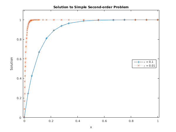
Example
This example solves the problem (written as a first-order system)
with boundary conditions
for the cases
and
using the default initial mesh in the first case, and the final mesh of the first case as initial mesh for the second (more difficult) case. We give the solution and the error at each mesh point to illustrate the accuracy of the method given the accuracy request
.
Note the call to
nag_file_set_unit_advisory (x04ab) prior to the call to
nag_ode_bvp_fd_lin_gen (d02gb).
Open in the MATLAB editor:
d02gb_example
function d02gb_example
fprintf('d02gb example results\n\n');
global eps;
mnp = int64(70);
a = 0;
b = 1;
tol = 0.001;
c = [1, 0; 0, 0];
d = [0, 0; 1, 0];
gam = [0; 1];
x = zeros(1,mnp);
np = int64(0);
n = int64(2);
xkeep = zeros(1,2);
npkeep = zeros(2);
ykeep = zeros(1,2);
espkeep = zeros(2);
for i = 1:2
eps = 10^(-i);
[c, d, gam, x, y, np, ifail] = ...
d02gb(a, b, tol, @f, @g, c, d, gam, x, np, 'n', n, 'mnp', mnp);
for j = 1:np
xkeep(j,i) = x(j);
ykeep(j,i) = y(1,j);
end
npkeep(i) = np;
espkeep(i) = eps;
fprintf(' for eps = %7.4f, number of points required, np = %d\n', eps, np);
end
fig1 = figure;
plot(xkeep(1:npkeep(1),1), ykeep(1:npkeep(1),1), '-+', ...
xkeep(1:npkeep(2),2), ykeep(1:npkeep(2),2), ':x');
set(gca, 'YLim', [0 1.1]);
set(gca, 'XLim', [-0.01 1.01]);
title('Solution to Simple Second-order Problem');
xlabel('x');
ylabel('Solution');
legend(['\epsilon = ', num2str(espkeep(1))], ...
['\epsilon = ', num2str(espkeep(2))], 'Location', 'East');
function f = f(x)
global eps;
f=zeros(2,2);
f(1,2) = 1;
f(2,2) = -1/eps;
function g = g(x)
g=zeros(2,1);
d02gb example results

 for eps =  0.1000, number of points required, np = 15
 for eps =  0.0100, number of points required, np = 49
PDF version (NAG web site
, 64-bit version, 64-bit version)
© The Numerical Algorithms Group Ltd, Oxford, UK. 2009–2015