NAG Library Chapter Introduction
G07 (univar)
Univariate Estimation
1
Scope of the Chapter
This chapter deals with the estimation of unknown parameters of a univariate distribution. It includes both point and interval estimation using maximum likelihood and robust methods.
2
Background to the Problems
Statistical inference is concerned with the making of inferences about a population using the observed part of the population called a sample. The population can usually be described using a probability model which will be written in terms of some unknown parameters. For example, the hours of relief given by a drug may be assumed to follow a Normal distribution with mean and variance ; it is then required to make inferences about the parameters, and , on the basis of an observed sample of relief times.
There are two main aspects of statistical inference: the
estimation of the parameters and the
testing of hypotheses about the parameters. In the example above, the values of the parameter
may be estimated and the hypothesis that
tested. This chapter is mainly concerned with estimation but the test of a hypothesis about a parameter is often closely linked to its estimation. Tests of hypotheses which are not linked closely to estimation are given in the chapter on nonparametric statistics (
Chapter G08).
There are two types of estimation to be considered in this chapter: point estimation and interval estimation. Point estimation is when a single value is obtained as the best estimate of the parameter. However, as this estimate will be based on only one of a large number of possible samples, it can be seen that if a different sample were taken, a different estimate would be obtained. The distribution of the estimate across all the possible samples is known as the sampling distribution. The sampling distribution contains information on the performance of the estimator, and enables estimators to be compared. For example, a good estimator would have a sampling distribution with mean equal to the true value of the parameter; that is, it should be an unbiased estimator; also the variance of the sampling distribution should be as small as possible. When considering a parameter estimate it is important to consider its variability as measured by its variance, or more often the square root of the variance, the standard error.
The sampling distribution can be used to find interval estimates or confidence intervals for the parameter. A confidence interval is an interval calculated from the sample so that its distribution, as given by the sampling distribution, is such that it contains the true value of the parameter with a certain probability.
Estimates will be functions of the observed sample and these functions are known as
estimators. It is usually more convenient for the estimator to be based on statistics from the sample rather than all the individuals observations. If these statistics contain all the relevant information then they are known as
sufficient statistics. There are several ways of obtaining the estimators; these include least squares, the method of moments, and
maximum likelihood. Least squares estimation requires no knowledge of the distributional form of the error apart from its mean and variance matrix, whereas the method of maximum likelihood is mainly applicable to situations in which the true distribution is known apart from the values of a finite number of unknown parameters. Note that under the assumption of Normality, the least squares estimation is equivalent to the maximum likelihood estimation. Least squares is often used in regression analysis as described in
Chapter G02, and maximum likelihood is described below.
Estimators derived from least squares or maximum likelihood will often be greatly affected by the presence of extreme or unusual observations. Estimators that are designed to be less affected are known as robust estimators.
2.1
Maximum Likelihood Estimation
Let
be a univariate random variable with probability density function
where
is a vector of length
consisting of the unknown parameters. For example, a Normal distribution with mean
and standard deviation
has probability density function
The likelihood for a sample of
independent observations is
where
is the observed value of
. If each
has an identical distribution, this reduces to
and the log-likelihood is
The maximum likelihood estimates (
) of
are the values of
that maximize
(1) and
(2). If the range of
is independent of the parameters, then
can usually be found as the solution to
Note that
is known as the efficient score.
Maximum likelihood estimators possess several important properties.
| (a) |
Maximum likelihood estimators are functions of the sufficient statistics. |
| (b) |
Maximum likelihood estimators are (under certain conditions) consistent. That is, the estimator converges in probability to the true value as the sample size increases. Note that for small samples the maximum likelihood estimator may be biased. |
| (c) |
For maximum likelihood estimators found as a solution to (3), subject to certain conditions, it follows that
and
and then that is asymptotically Normal with mean vector and variance-covariance matrix where denotes the true value of . The matrix is known as the information matrix and is known as the Cramer–Rao lower bound for the variance of an estimator of . |
For example, if we consider a sample,
, of size
drawn from a Normal distribution with unknown mean
and unknown variance
then we have
and thus
and
Then equating these two equations to zero and solving gives the maximum likelihood estimates
and
These maximum likelihood estimates are asymptotically Normal with mean vector
, where
and covariance matrix
. To obtain
we find the second derivatives of
with respect to
and
as follows:
Then
so that
To obtain an estimate of
the matrix may be evaluated at the maximum likelihood estimates.
It may not always be possible to find maximum likelihood estimates in a convenient closed form, and in these cases iterative numerical methods, such as the Newton–Raphson procedure or the EM algorithm (expectation maximization), will be necessary to compute the maximum likelihood estimates. Their asymptotic variances and covariances may then be found by substituting the estimates into the second derivatives. Note that it may be difficult to find the expected value of the second derivatives required for the variance-covariance matrix and in these cases the observed value of the second derivatives is often used.
The use of maximum likelihood estimation allows the construction of generalized likelihood ratio tests. If
, where
is the maximized log-likelihood function for a model
and
is the maximized log-likelihood function for a model
, then under the hypothesis that model
is correct,
is asymptotically distributed as a
variable with
degrees of freedom. Consider two models in which model
has
parameters and model
is a sub-model (nested model) of model
with
parameters, that is model
has an extra
parameters. This result provides a useful method for performing hypothesis tests on the parameters. Alternatively, tests exist based on the asymptotic Normality of the estimator and the efficient score; see page 315 of
Cox and Hinkley (1974).
2.2
Confidence Intervals
Suppose we can find a function,
, whose distribution depends upon the sample
but not on the unknown parameter
, and which is a monotonic (say decreasing) function in
for each
, then we can find
such that
no matter what
happens to be. The function
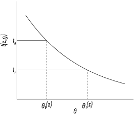
is known as a pivotal quantity. Since the function is monotonic the statement that
may be rewritten as
see
Figure 1. The statistic
will vary from sample to sample and if we assert that
for any sample values which arise, we will be right in a proportion
of the cases, in the long run or on average. We call
a
upper confidence limit for
.
We have considered only an upper confidence limit. The above idea may be generalized to a two-sided confidence interval where two quantities, and , are found such that for all , . This interval may be rewritten as . Thus if we assert that lies in the interval [] we will be right on average in proportion of the times under repeated sampling.
Hypothesis (significance) tests on the parameters may be used to find these confidence limits. For example, if we observe a value, , from a binomial distribution, with known parameter and unknown parameter , then to find the lower confidence limit we find such that the probability that the null hypothesis : (against the one sided alternative that ) will be rejected, is less than or equal to . Thus for a binomial random variable, , with parameters and we require that . The upper confidence limit, , can be constructed in a similar way.
For large samples the asymptotic Normality of the maximum likelihood estimates discussed above is used to construct confidence intervals for the unknown parameters.
2.3
Robust Estimation
For particular cases the probability density function can be written as
for a suitable function
; then
is known as a location parameter and
, usually written as
, is known as a scale parameter. This is true of the Normal distribution.
If
is a location parameter, as described above, then equation
(3) becomes
where
.
For the scale parameter
(or
) the equation is
where
.
For the Normal distribution
and
. Thus, the maximum likelihood estimates for
and
are the sample mean and variance with the
divisor respectively. As the latter is biased,
(7) can be replaced by
where
is a suitable constant, which for the Normal
function is
.
The influence of an observation on the estimates depends on the form of the
and
functions. For a discussion of influence, see
Hampel et al. (1986) and
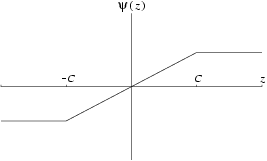
Huber (1981). The influence of extreme values can be reduced by bounding the values of the
- and
-functions. One suggestion due to
Huber (1981) is
Figure 2
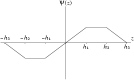
Redescending
-functions are often considered; these give zero values to
for large positive or negative values of
.
Hampel et al. (1986) suggested
Figure 3
Usually a -function based on Huber's -function is used: . Estimators based on such bounded -functions are known as -estimators, and provide one type of robust estimator.
Other robust estimators for the location parameter are
| (i) |
the sample median, |
| (ii) |
the trimmed mean, i.e., the mean calculated after the extreme values have been removed from the sample, |
| (iii) |
the winsorized mean, i.e., the mean calculated after the extreme values of the sample have been replaced by other more moderate values from the sample. |
For the scale parameter, alternative estimators are
| (i) |
the median absolute deviation scaled to produce an estimator which is unbiased in the case of data coming from a Normal distribution, |
| (ii) |
the winsorized variance, i.e., the variance calculated after the extreme values of the sample have been replaced by other more moderate values from the sample. |
For a general discussion of robust estimation, see
Hampel et al. (1986) and
Huber (1981).
2.4
Robust Confidence Intervals
In
Section 2.2 it was shown how tests of hypotheses can be used to find confidence intervals. That approach uses a parametric test that requires the assumption that the data used in the computation of the confidence has a known distribution. As an alternative, a more robust confidence interval can be found by replacing the parametric test by a nonparametric test. In the case of the confidence interval for the location parameter, a Wilcoxon test statistic can be used, and for the difference in location, computed from two samples, a Mann–Whitney test statistic can be used.
3
Recommendations on Choice and Use of Available Routines
Maximum Likelihood Estimation and Confidence Intervals
g07aaf provides a confidence interval for the parameter
of the binomial distribution.
g07abf provides a confidence interval for the mean parameter of the Poisson distribution.
g07bbf provides maximum likelihood estimates and their standard errors for the parameters of the Normal distribution from grouped and/or censored data.
g07bef provides maximum likelihood estimates and their standard errors for the parameters of the Weibull distribution from data which may be right-censored.
g07bff provides maximum likelihood estimates and their standard errors for the parameters of the generalized Pareto distribution.
g07caf provides a
-test statistic to test for a difference in means between two Normal populations, together with a confidence interval for the difference between the means.
Robust Estimation
g07dbf provides
-estimates for location and, optionally, scale using four common forms of the
-function.
g07dcf produces the
-estimates for location and, optionally, scale but for user-supplied
- and
-functions.
g07daf provides the sample median, median absolute deviation, and the scaled value of the median absolute deviation.
g07ddf provides the trimmed mean and winsorized mean together with estimates of their variance based on a winsorized variance.
Robust Internal Estimation
g07eaf produces a rank based confidence interval for locations.
g07ebf produces a rank based confidence interval for the difference in location between two populations.
Outlier Detection
This chapter provides two routines for identifying potential outlying values,
g07gaf and
g07gbf. Many of the model fitting routines, for examples those in
Chapters G02 and
G13 also return vectors of residuals which can also be used to aid in the identification of outlying values.
4
Functionality Index
| Confidence intervals for parameters, | | |
| Maximum likelihood estimation of parameters, | | |
| Normal distribution, grouped and/or censored data | | g07bbf |
| raw data or single variance supplied | | g07gaf |
| generalized Pareto distribution | | g07bff |
| median, median absolute deviation and robust standard deviation | | g07daf |
| M-estimates for location and scale parameters, | | |
| standard weight functions | | g07dbf |
| trimmed and winsorized means and estimates of their variance | | g07ddf |
| user-defined weight functions | | g07dcf |
5
Auxiliary Routines Associated with Library Routine Arguments
None.
6
Routines Withdrawn or Scheduled for Withdrawal
None.
7
References
Cox D R and Hinkley D V (1974) Theoretical Statistics Chapman and Hall
Hampel F R, Ronchetti E M, Rousseeuw P J and Stahel W A (1986) Robust Statistics. The Approach Based on Influence Functions Wiley
Huber P J (1981) Robust Statistics Wiley
Kendall M G and Stuart A (1973) The Advanced Theory of Statistics (Volume 2) (3rd Edition) Griffin
Silvey S D (1975) Statistical Inference Chapman and Hall


